See this [video][pack-vid] for step-by-step instruction on how to install, use and update packages from CRAN
R Packages
R packages
The base installation of R comes with many useful packages as standard. These packages will contain many of the functions you will use on a daily basis. However, as you start using R for more diverse projects (and as your own use of R evolves) you will find that there comes a time when you will need to extend R’s capabilities. Happily, many thousands of R users have developed useful code and shared this code as installable packages. You can think of a package as a collection of functions, data and help files collated into a well defined standard structure which you can download and install in R. These packages can be downloaded from a variety of sources but the most popular are [CRAN][cran-packages], [Bioconductor][bioconductor] and [GitHub][github]. Currently, CRAN hosts over 15000 packages and is the official repository for user contributed R packages. Bioconductor provides open source software oriented towards bioinformatics and hosts over 1800 R packages. GitHub is a website that hosts git repositories for all sorts of software and projects (not just R). Often, cutting edge development versions of R packages are hosted on GitHub so if you need all the new bells and whistles then this may be an option. However, a potential downside of using the development version of an R package is that it might not be as stable as the version hosted on CRAN (it’s in development!) and updating packages won’t be automatic.
CRAN packages
To install a package from CRAN you can use the install.packages() function. For example if you want to install the remotes package enter the following code into the Console window of RStudio (note: you will need a working internet connection to do this)
install.packages('remotes', dependencies = TRUE)You may be asked to select a CRAN mirror, just select ‘0-cloud’ or a mirror near to your location. The dependencies = TRUE argument ensures that additional packages that are required will also be installed.
It’s good practice to occasionally update your previously installed packages to get access to new functionality and bug fixes. To update CRAN packages you can use the update.packages() function (you will need a working internet connection for this).
update.packages(ask = FALSE)The ask = FALSE argument avoids having to confirm every package download which can be a pain if you have many packages installed.
Bioconductor packages
To install packages from Bioconductor the process is a [little different][bioc-install]. You first need to install the BiocManager package. You only need to do this once unless you subsequently reinstall or upgrade R.
install.packages('BiocManager', dependencies = TRUE)Once the BiocManager package has been installed you can either install all of the ‘core’ Bioconductor packages with
BiocManager::install()or install specific packages such as the ‘GenomicRanges’ and ‘edgeR’ packages.
BiocManager::install(c("GenomicRanges", "edgeR"))To update Bioconductor packages just use the BiocManager::install() function again.
BiocManager::install(ask = FALSE)Again, you can use the ask = FALSE argument to avoid having to confirm every package download.
GitHub packages
There are multiple options for installing packages hosted on GitHub. Perhaps the most efficient method is to use the install_github() function from the remotes package (you installed this package previously). Before you use the function you will need to know the GitHub username of the repository owner and also the name of the repository. For example, the development version of dplyr from Hadley Wickham is hosted on the tidyverse GitHub account and has the repository name ‘dplyr’ (just Google ‘github dplyr’). To install this version from GitHub, use
remotes::install_github('tidyverse/dplyr')The safest way (that we know of) to update a package installed from GitHub is to just reinstall it using the above command.
Using packages
Once you have installed a package onto your computer it is not immediately available for you to use. To use a package you first need to load the package by using the library() function. For example, to load the remotes package you previously installed.
library(remotes)The library() function will also load any additional packages required and may print out additional package information. It is important to realise that every time you start a new R session (or restore a previously saved session) you need to load the packages you will be using. We tend to put all our library() statements required for our analysis near the top of our R scripts to make them easily accessible and easy to add to as our code develops. If you try to use a function without first loading the relevant R package you will receive an error message that R could not find the function. For example, if you try to use the install_github() function without loading the remotes package first you will receive the following error.
install_github('tidyverse/dplyr')

# Error in install_github("tidyverse/dplyr") :
#  could not find function "install_github"
Sometimes it can be useful to use a function without first using the library() function. If, for example, you will only be using one or two functions in your script and don’t want to load all of the other functions in a package then you can access the function directly by specifying the package name followed by two colons and then the function name.
remotes::install_github('tidyverse/dplyr')This is how we were able to use the install() and install_github() functions above without first loading the packages BiocManager and remotes. Most of the time we recommend using the library() function.
Projects in RStudio
As with most things in life, when it comes to dealing with data and data analysis things are so much simpler if you’re organised. Clear project organisation makes it easier for both you (especially the future you) and your collaborators to make sense of what you’ve done. There’s nothing more frustrating than coming back to a project months (sometimes years) later and have to spend days (or weeks) figuring out where everything is, what you did and why you did it. A well documented project that has a consistent and logical structure increases the likelihood that you can pick up where you left off with minimal fuss no matter how much time has passed. In addition, it’s much easier to write code to automate tasks when files are well organised and are sensibly named. This is even more relevant nowadays as it’s never been easier to collect vast amounts of data which can be saved across 1000’s or even 100,000’s of separate data files. Lastly, having a well organised project reduces the risk of introducing bugs or errors into your workflow and if they do occur (which inevitably they will at some point), it makes it easier to track down these errors and deal with them efficiently.
Thankfully, there are some nice features in R and RStudio that make it quite easy to manage a project. There are also a few simple steps you can take right at the start of any project to help keep things shipshape.
A great way of keeping things organised is to use RStudio Projects. An RStudio Project keeps all of your R scripts, R markdown documents, R functions and data together in one place. The nice thing about RStudio Projects is that each project has its own directory, workspace, history and source documents so different analyses that you are working on are kept completely separate from each other. This means that you can have multiple instances of RStudio open at the same time (if that’s your thing) or you can very easily switch between projects without fear of them interfering with each other.
See this [video][rstudio-prog-vid] for step-by-step instructions on how to create and work with RStudio projects
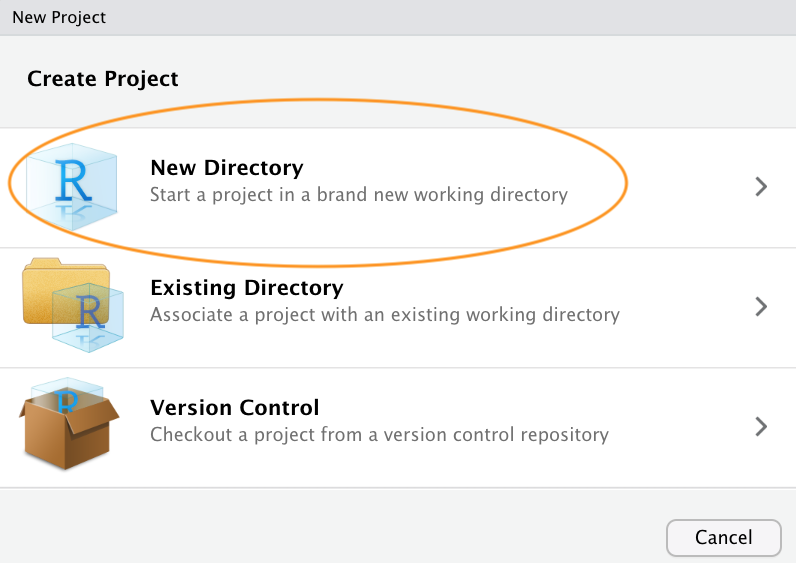
To create a project, open RStudio and select File -> New Project... from the menu. You can create either an entirely new project, a project from an existing directory or a version controlled project (see the GitHub Chapter for further details about this). In this Chapter we will create a project in a new directory.
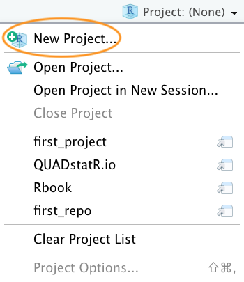
You can also create a new project by clicking on the ‘Project’ button in the top right of RStudio and selecting ‘New Project…’
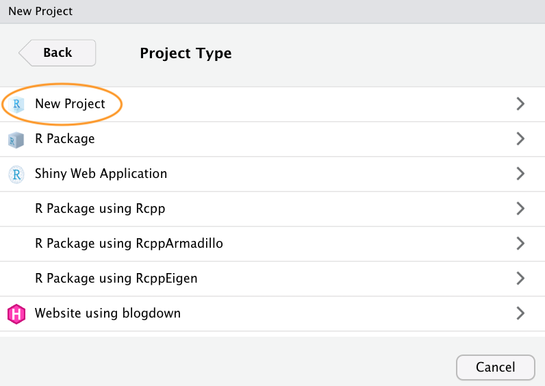
In the next window select ‘New Project’.
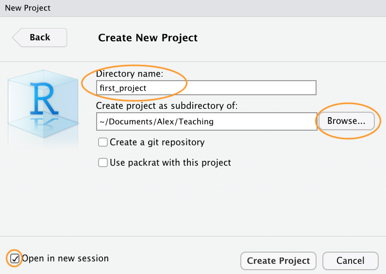
Now enter the name of the directory you want to create in the ‘Directory name:’ field (we’ll call it first_project for this Chapter). If you want to change the location of the directory on your computer click the ‘Browse…’ button and navigate to where you would like to create the directory. We always tick the ‘Open in new session’ box as well. Finally, hit the ‘Create Project’ to create the new project.
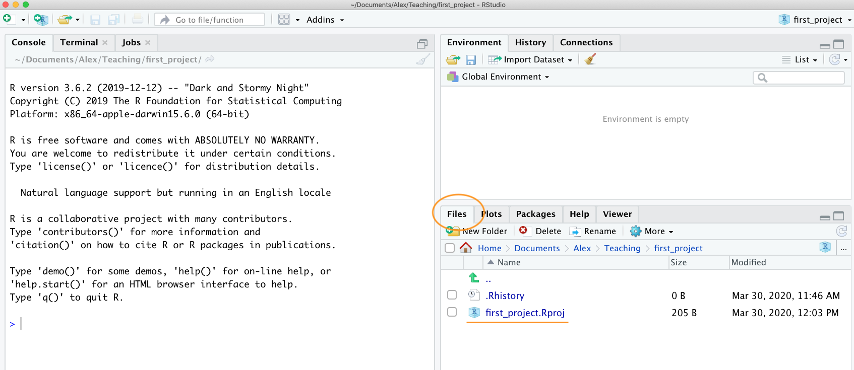
Once your new project has been created you will now have a new folder on your computer that contains an RStudio project file called first_project.Rproj. This .Rproj file contains various project options (but you shouldn’t really interact with it) and can also be used as a shortcut for opening the project directly from the file system (just double click on it). You can check this out in the ‘Files’ tab in RStudio (or in Finder if you’re on a Mac or File Explorer in Windows).
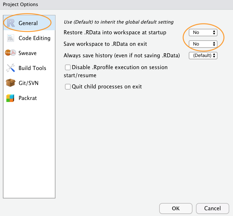
The last thing we suggest you do is select Tools -> Project Options... from the menu. Click on the ‘General’ tab on the left hand side and then change the values for ‘Restore .RData into workspace at startup’ and ‘Save workspace to .RData on exit’ from ‘Default’ to ‘No’. This ensures that every time you open your project you start with a clean R session. You don’t have to do this (many people don’t) but we prefer to start with a completely clean workspace whenever we open our projects to avoid any potential conflicts with things we have done in previous sessions. The downside to this is that you will need to rerun your R code every time you open your project.
Now that you have an RStudio project set up you can start creating R scripts (or R markdown documents) or whatever you need to complete you project. All of the R scripts will now be contained within the RStudio project and saved in the project folder.
Working directories
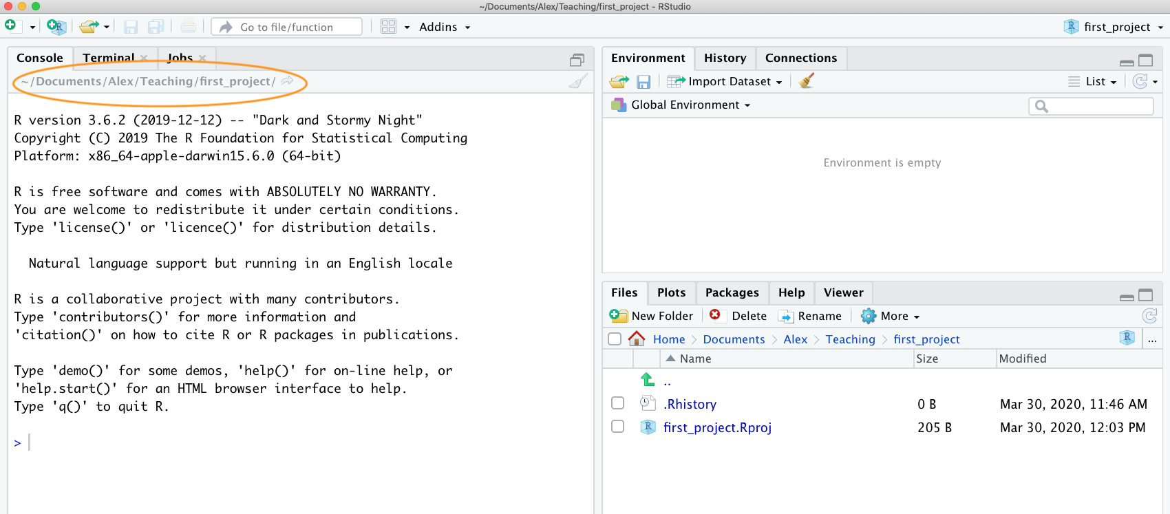
The working directory is the default location where R will look for files you want to load and where it will put any files you save. One of the great things about using RStudio Projects is that when you open a project it will automatically set your working directory to the appropriate location. You can check the file path of your working directory by looking at bar at the top of the Console pane. Note: the ~ symbol above is shorthand for /Users/nhy163/ on a Mac computer (the same on Linux computers).
You can also use the getwd() function in the Console which returns the file path of the current working directory.
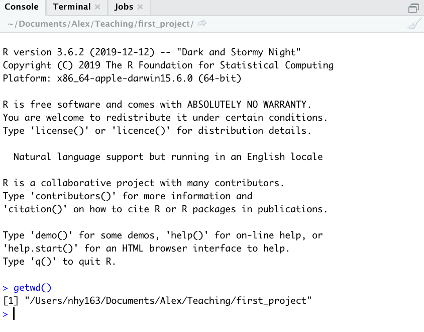
In the example above, the working directory is a folder called ‘first_project’ which is a subfolder of “Teaching’ in the ‘Alex’ folder which in turn is in a ‘Documents’ folder located in the ‘nhy163’ folder which itself is in the ‘Users’ folder. On a Windows based computer our working directory would also include a drive letter (i.e. C:/Users/nhy163/Documents/Alex/Teaching/first_project).
If you weren’t using an RStudio Project then you would have to set your working directory using the setwd() function at the start of every R script (something we did for many years).
setwd('/Users/nhy163/Documents/Alex/Teaching/first_project')However, the problem with setwd() is that it uses an absolute file path which is specific to the computer you are working on. If you want to send your script to someone else (or if you’re working on a different computer) this absolute file path is not going to work on your friend/colleagues computer as their directory configuration will be different (you are unlikely to have a directory structure /Users/nhy163/Documents/Alex/Teaching/ on your computer). This results in a project that is not self-contained and not easily portable. RStudio solves this problem by allowing you to use relative file paths which are relative to the Root project directory. The Root project directory is just the directory that contains the .Rproj file (first_project.Rproj in our case). If you want to share your analysis with someone else, all you need to do is copy the entire project directory and send to your to your collaborator. They would then just need to open the project file and any R scripts that contain references to relative file paths will just work. For example, let’s say that you’ve created a subdirectory called raw_data in your Root project directory that contains a tab delimited datafile called mydata.txt (we will cover directory structures below). To import this datafile in an RStudio project using the read.table() function (don’t worry about this now, we will cover this in much more detail in Chapter 3) all you need to include in your R script is
dataf <- read.table('raw_data/mydata.txt', header = TRUE,
                      sep = '\t')
Because the file path raw_data/mydata.txt is relative to the project directory it doesn’t matter where you collaborator saves the project directory on their computer it will still work.
If you weren’t using an RStudio project then you would have to use either of the options below neither of which would work on a different computer.
setwd('/Users/nhy163/Documents/Alex/Teaching/first_project/')

dataf <- read.table('raw_data/mydata.txt', header = TRUE, sep = '\t')

# or

dataf <- read.table('/Users/nhy163/Documents/Alex/Teaching/first_project/raw_data/mydata.txt', header = TRUE, sep = '\t')
For those of you who want to take the notion of relative file paths a step further, take a look at the here() function in the here [package][here]. The here() function allows you to automagically build file paths for any file relative to the project root directory that are also operating system agnostic (works on a Mac, Windows or Linux machine). For example, to import our mydata.txt file from the raw_data directory just use
library(here)  # you may need to install the here package first
dataf <- read.table(here("raw_data", "mydata.txt"),
                     header = TRUE, sep = '\t',
                    stringsAsFactors = TRUE)

# or without loading the here package

dataf <- read.table(here::here("raw_data", "mydata.txt"),
                      header = TRUE, sep = '\t',
                      stringsAsFactors = TRUE)