Directory Configuration

Author

Mahesh Divakaran & Dr. Jayadevan Sreedharan

Directory structure

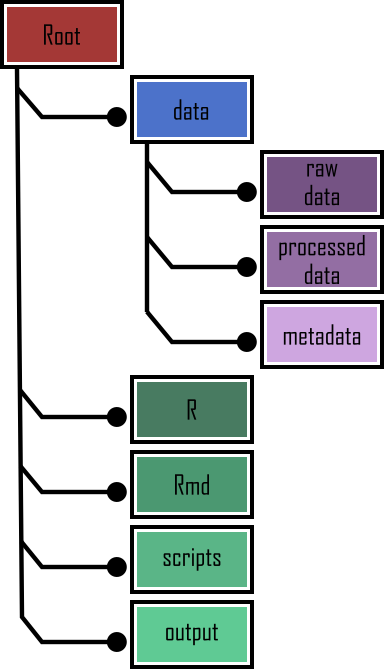
In addition to using RStudio Projects, it’s also really good practice to structure your working directory in a consistent and logical way to help both you and your collaborators. We frequently use the following directory structure in our R based projects

In our working directory we have the following directories:

Root - This is your project directory containing your .Rproj file.
data - We store all our data in this directory. The subdirectory called raw_data contains raw data files and only raw data files. These files should be treated as read only and should not be changed in any way. If you need to process/clean/modify your data do this in R (not MS Excel) as you can document (and justify) any changes made. Any processed data should be saved to a separate file and stored in the processed_data subdirectory. Information about data collection methods, details of data download and any other useful metadata should be saved in a text document (see README text files below) in the metadata subdirectory.
R - This is an optional directory where we save all of the custom R functions we’ve written for the current analysis. These can then be sourced into R using the source() function.
Rmd - An optional directory where we save our R markdown documents.
scripts - All of the main R scripts we have written for the current project are saved here.
output - Outputs from our R scripts such as plots, HTML files and data summaries are saved in this directory. This helps us and our collaborators distinguish what files are outputs and which are source files.

Of course, the structure described above is just what works for us most of the time and should be viewed as a starting point for your own needs. We tend to have a fairly consistent directory structure across our projects as this allows us to quickly orientate ourselves when we return to a project after a while. Having said that, different projects will have different requirements so we happily add and remove directories as required.

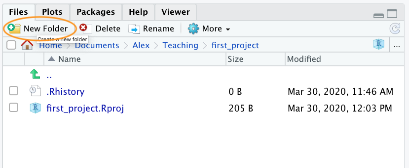
You can create your directory structure using Windows Explorer (or Finder on a Mac) or within RStudio by clicking on the ‘New folder’ button in the ‘Files’ pane.

An alternative approach is to use the dir.create() and list.files() functions in the R Console.

# create directory called 'data'
dir.create('data')

# create subdirectory raw_data in the data directory
dir.create('data/raw_data')

# list the files and directories
list.files(recursive = TRUE, include.dirs = TRUE)

# [1] "data"  "data/raw_data"   "first_project.Rproj"

File names

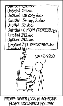
What you call your files matters more than you might think. Naming files is also more difficult than you think. The key requirement for a ‘good’ file name is that it’s informative whilst also being relatively short. This is not always an easy compromise and often requires some thought. Ideally you should try to avoid the following!

Although there’s not really a recognised standard approach to naming files (actually [there is][file_wiki], just not everyone uses it), there are a couple of things to bear in mind.

First, avoid using spaces in file names by replacing them with underscores or even hyphens. Why does this matter? One reason is that some command line software (especially many bioinformatic tools) won’t recognise a file name with a space and you’ll have to go through all sorts of shenanigans using escape characters to make sure spaces are handled correctly. Even if you don’t think you will ever use command line software you may be doing so indirectly. Take R markdown for example, if you want to render an R markdown document to pdf using the rmarkdown package you will actually be using a command line LaTeX engine under the hood (called [Pandoc][pandoc]). Another good reason not to use spaces in file names is that it makes searching for file names (or parts of file names) using [regular expressions][regex] in R (or any other language) much more difficult.
For the reasons given above, also avoid using special characters (i.e. @£$%^&*(:/) in your file names.
If you are versioning your files with sequential numbers (i.e. file1, file2, file3 …) and you have more than 9 files you should use 01, 02, 03 .. 10 as this will ensure the files are printed in the correct order (see what happens if you don’t). If you have more than 99 files then use 001, 002, 003… etc.
If your file names include dates, use the ISO 8601 format YYYY-MM-DD (or YYYYMMDD) to ensure your files are listed in proper chronological order.
Never use the word final in any file name - it never is!

Whatever file naming convention you decide to use, try to adopt early, stick with it and be consistent. You’ll thank us!

Project documentation

A quick note or two about writing R code and creating R scripts. Unless you’re doing something really quick and dirty we suggest that you always write your R code as an R script. R scripts are what make R so useful. Not only do you have a complete record of your analysis, from data manipulation, visualisation and statistical analysis, you can also share this code (and data) with friends, colleagues and importantly when you submit and publish your research to a journal. With this in mind, make sure you include in your R script all the information required to make your work reproducible (author names, dates, sampling design etc). This information could be included as a series of comments # or, even better, by mixing executable code with narrative into an R markdown document. It’s also good practice to include the output of the sessionInfo() function at the end of any script which prints the R version, details of the operating system and also loaded packages. A really good alternative is to use the session_info() function from the xfun package for a more concise summary of our session environment.

Here’s an example of including meta-information at the start of an R script.

# Title: Time series analysis of snouters

# Purpose : This script performs a time series analyses on 
#           snouter count data.
#           Data consists of counts of snouter species 
#           collected from 18 islands in the Hy-yi-yi 
#           archipelago between 1950 and 1957. 
#           For details of snouter biology see:
#           https://en.wikipedia.org/wiki/Rhinogradentia

# Project number: #007

# DataFile:'data/snouter_pop.txt'

# Author: A. Nother
# Contact details: a.nother@uir.ac.uk

# Date script created: Mon Dec 2 16:06:44 2019 -----------
# Date script last modified: Thu Dec 12 16:07:12 2019 ----

# package dependencies
library(PopSnouter)
library(ggplot2)

print('put your lovely R code here')

# good practice to include session information

xfun::session_info()

This is just one example and there are no hard and fast rules so feel free to develop a system that works for you. A really useful shortcut in RStudio is to automatically include a time and date stamp in your R script. To do this, write ts where you want to insert your time stamp in your R script and then press the ‘shift + tab’ keys. RStudio will magically convert ts into the current date and time and also automatically comment out this line with a #. Another really useful RStudio shortcut is to comment out multiple lines in your script with a # symbol. To do this, highlight the lines of text you want to comment and then press ‘ctrl + shift + c’ (or ‘cmd + shift + c’ on a mac). To uncomment the lines just use ‘ctrl + shift + c’ again.

In addition to including metadata in your R scripts it’s also common practice to create a separate text file to record important information. By convention these text files are named README. We often include a README file in the directory where we keep our raw data. In this file we include details about when data were collected (or downloaded), how data were collected, information about specialised equipment, preservation methods, type and version of any machines used (i.e. sequencing equipment) etc. You can create a README file for your project in RStudio by clicking on the File -> New File -> Text File menu.

R style guide

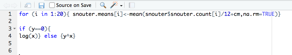
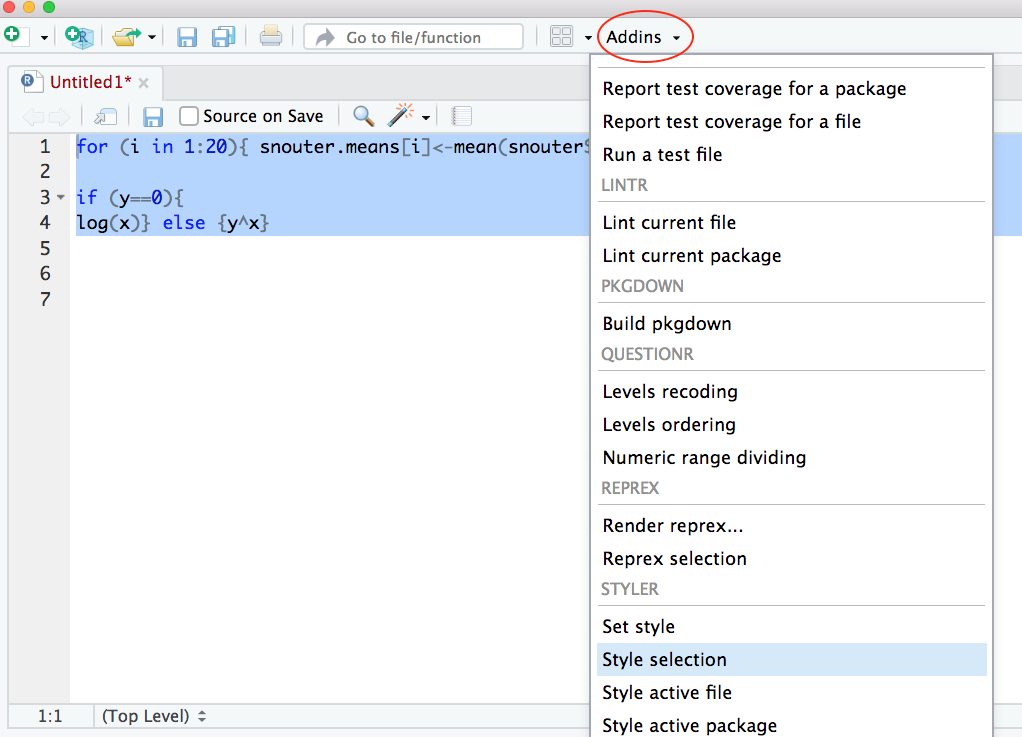
How you write your code is more or less up to you although your goal should be to make it as easy to read as possible (for you and others). Whilst there are no rules (and no code police), we encourage you to get into the habit of writing readable R code by adopting a particular style. We suggest that you follow Google’s [R style guide][style-google] whenever possible. This style guide will help you decide where to use spaces, how to indent code and how to use square [ ] and curly { } brackets amongst other things. If all that sounds like too much hard work you can install the styler package which includes an RStudio add-in to allow you to automatically restyle selected code (or entire files and projects) with the click of your mouse. You can find more information about the styler package including how to install [here][styler]. Once installed, you can highlight the code you want to restyle, click on the ‘Addins’ button at the top of RStudio and select the ‘Style Selection’ option. Here is an example of poorly formatted R code.

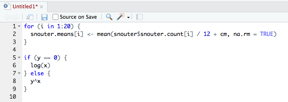
Now highlight the code and use the styler package to reformat

To produce some nicely formatted code

Backing up projects

Don’t be that person who loses hard won (and often expensive) data and analyses. Don’t be that person who thinks it’ll never happen to me - it will! Always think of the absolute worst case scenario, something that makes you wake up in a cold sweat at night, and do all you can to make sure this never happens. Just to be clear, if you’re relying on copying your precious files to an external hard disk or USB stick this is NOT an effective backup strategy. These things go wrong all the time as you lob them into your rucksack or ‘bag for life’ and then lug them between your office and home. Even if you do leave them plugged into your computer what happens when the building burns down (we did say worst case!)?

Ideally, your backups should be offsite and incremental. Happily there are numerous options for backing up your files. The first place to look is in your own institute. Most (all?) Universities have some form of network based storage that should be easily accessible and is also underpinned by a comprehensive disaster recovery plan. Other options include cloud based services such as Google Drive and Dropbox (to name but a few), but make sure you’re not storing sensitive data on these services and are comfortable with the often eye watering privacy policies.

Whilst these services are pretty good at storing files, they don’t really help with incremental backups. Finding previous versions of files often involves spending inordinate amounts of time trawling through multiple files named ‘final.doc’, ‘final_v2.doc’ and ‘final_usethisone.doc’ etc until you find the one you were looking for. The best way we know for both backing up files and managing different versions of files is to use Git and GitHub. To find out more about how you can use RStudio, Git and GitHub together see the Git and GitHub Chapter.