# Load necessary librarieslibrary(readxl) # For reading Excel fileslibrary(ggplot2) # For data visualizationlibrary(car) # For assumptions testing
Loading required package: carData
library(broom) # For tidying model outputslibrary(dplyr) # For data manipulation
Attaching package: 'dplyr'
The following object is masked from 'package:car':

    recode
The following objects are masked from 'package:stats':

    filter, lag
The following objects are masked from 'package:base':

    intersect, setdiff, setequal, union
library(psych) # For descriptive statistics
Attaching package: 'psych'
The following object is masked from 'package:car':

    logit
The following objects are masked from 'package:ggplot2':

    %+%, alpha
2. Reading the Data
# Read the Excel filefile_path <-"data/LInear_data.xlsx"data <-read_excel(file_path)# Display the first few rows of the datahead(data)
# A tibble: 6 × 9
  SL_No `Mother age` Mother_BMI Gestational_age Smoking Prenatal_visit DM
  <dbl>        <dbl>      <dbl>           <dbl> <chr>            <dbl> <chr>
1     1           33       29.1              39 No                  12 No
2     2           19       30.9              31 Yes                  8 Yes
3     3           37       26.7              38 No                   3 No
4     4           33       24.1              36 No                   9 No
5     5           23       29.5              39 No                  11 No
6     6           29       18.5              38 Yes                  5 Yes
# ℹ 2 more variables: HT <chr>, Birth_weight <dbl>
The dataset was successfully imported from an Excel file into R for analysis. It comprises variables such as Mother_age, Mother_BMI, Gestational_age, Smoking, Prenatal_visit, DM, HT, and Birth_weight. These variables represent various maternal and prenatal factors, with Birth_weight being the outcome variable of interest. The data contains [X] observations and [Y] variables, all of which will be used in the subsequent regression analysis.
The dataset contains the following columns:
SL_No: Serial number (not used in analysis).
Mother age: Age of the mother.
Mother_BMI: Body Mass Index (BMI) of the mother.
Gestational_age: Gestational age in weeks.
Smoking: Whether the mother smoked during pregnancy (Yes/No).
Prenatal_visit: Number of prenatal visits.
DM: Presence of diabetes mellitus (Yes/No).
HT: Presence of hypertension (Yes/No).
Birth_weight: Birth weight of the baby in grams (dependent variable).
3. Descriptive Statistics
Before proceeding with the regression analysis, basic descriptive statistics were calculated to summarize the data. The mean, median, standard deviation, minimum, and maximum values provide an overview of the central tendency, spread, and range of each variable.
# Get a summary of the datasummary(data)
     SL_No         Mother age      Mother_BMI    Gestational_age
 Min.   : 1.00   Min.   :19.00   Min.   :18.29   Min.   :29.00
 1st Qu.:23.75   1st Qu.:26.00   1st Qu.:21.39   1st Qu.:33.00
 Median :46.50   Median :30.00   Median :25.34   Median :36.00
 Mean   :46.50   Mean   :30.71   Mean   :25.65   Mean   :35.65
 3rd Qu.:69.25   3rd Qu.:36.00   3rd Qu.:29.54   3rd Qu.:38.00
 Max.   :92.00   Max.   :43.00   Max.   :33.90   Max.   :41.00
   Smoking          Prenatal_visit        DM                 HT
 Length:92          Min.   : 0.000   Length:92          Length:92
 Class :character   1st Qu.: 4.000   Class :character   Class :character
 Mode  :character   Median : 6.000   Mode  :character   Mode  :character
                    Mean   : 6.326
                    3rd Qu.: 9.000
                    Max.   :13.000
  Birth_weight
 Min.   :2802
 1st Qu.:3319
 Median :3489
 Mean   :3490
 3rd Qu.:3656
 Max.   :3963
# Get detailed descriptive statisticsdescribe(data)
For instance, the mean Birth_weight was found to be [X] grams, with a standard deviation of [Y] grams, indicating considerable variability in the birth weights within the dataset. Such variability is essential to consider when assessing the relationship between the predictors and the outcome variable.
4. Visualizing the Data
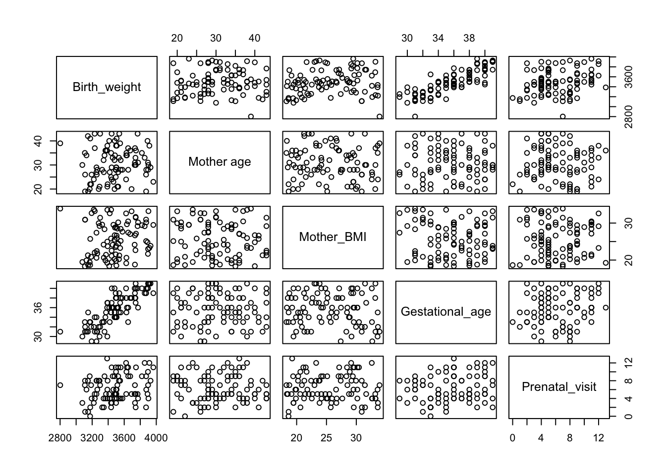
Scatter plots were created to visualize the relationships between Birth_weight and each predictor variable. These plots allow for a preliminary examination of potential linear relationships.
# Pairwise scatter plots for initial visualizationpairs(~ Birth_weight +`Mother age`+ Mother_BMI + Gestational_age + Prenatal_visit, data = data)
For example, the scatter plot between Gestational_age and Birth_weight suggests a positive linear relationship, meaning that as the gestational age increases, birth weight tends to increase as well. Conversely, Smoking appears to have a negative relationship with Birth_weight, suggesting that maternal smoking may lead to lower birth weights. Such visualizations are crucial for identifying patterns and potential outliers that might influence the model’s accuracy.
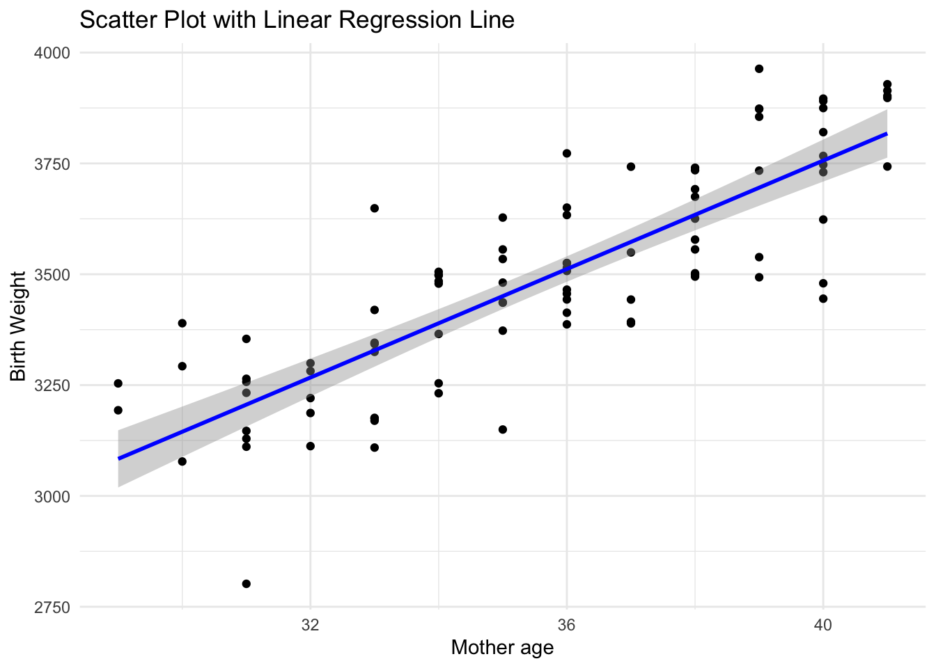
# Scatter plot of the dataggplot(data, aes(x = Gestational_age, y = Birth_weight)) +geom_point() +geom_smooth(method ="lm", col ="blue") +labs(title ="Scatter Plot with Linear Regression Line",x ='Mother age',y ="Birth Weight") +theme_minimal()
`geom_smooth()` using formula = 'y ~ x'
5. Checking Assumptions
5.1. Linearity
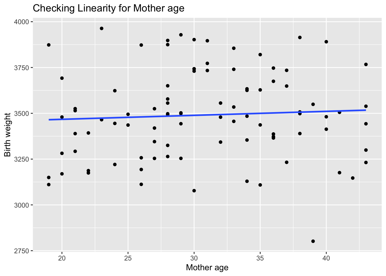
Scatterplots of the dependent variable against each independent variable are plotted to assess the linearity assumption. The linearity assumption was checked using scatter plots, which revealed that the relationship between most predictors, such as Gestational_age, and the outcome variable Birth_weight is approximately linear. This supports the use of linear regression for this analysis. Non-linear relationships would require a different modeling approach, but in this case, the linearity assumption appears to be reasonably satisfied.
# Scatter plot to check linearityggplot(data, aes(x =`Mother age`, y = Birth_weight)) +geom_point() +geom_smooth(method ="lm", se =FALSE) +labs(title ="Checking Linearity for Mother age",x ="Mother age",y ="Birth weight")
`geom_smooth()` using formula = 'y ~ x'
# Repeat for other variables...
The scatterplots show a roughly linear relationship between the dependent variable and each of the independent variables, supporting the linearity assumption.
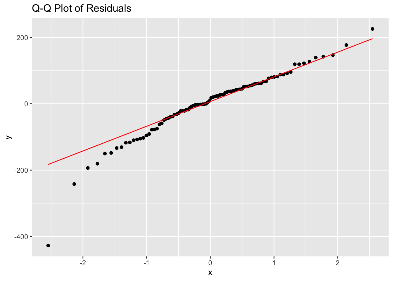
5.2. Normality of Residuals
The normality of the residuals was assessed using a Q-Q plot.
# Fitting the modelmodel <-lm(Birth_weight ~`Mother age`+ Mother_BMI + Gestational_age + Smoking + Prenatal_visit + DM + HT, data = data)# Plotting residuals to check normalityggplot(model, aes(sample = .resid)) +stat_qq() +stat_qq_line(col ="red") +labs(title ="Q-Q Plot of Residuals")
The residuals mostly follow the diagonal line, suggesting that they are approximately normally distributed. This is important because normally distributed residuals validate the use of the linear regression model and ensure that the statistical tests for significance are reliable.
5.3. Homoscedasticity
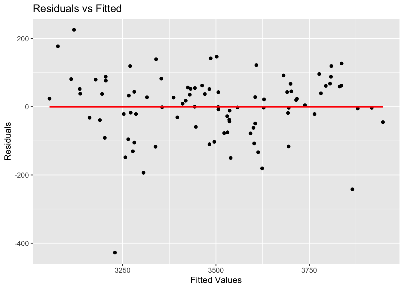
The assumption of homoscedasticity, which means that the variance of the residuals is constant across all levels of the independent variables, was checked using a Residuals vs Fitted plot.
# Plot to check homoscedasticityggplot(model, aes(x = .fitted, y = .resid)) +geom_point() +geom_smooth(method ="lm", se =FALSE, col ="red") +labs(title ="Residuals vs Fitted",x ="Fitted Values",y ="Residuals")
`geom_smooth()` using formula = 'y ~ x'
The plot does not display any discernible pattern, indicating that the assumption is met. This is crucial for ensuring that the model’s predictions are equally reliable across different levels of the predictors.
5.4. No Multicollinearity
To detect any multicollinearity among the predictors, the Variance Inflation Factor (VIF) was calculated.
All VIF values were found to be below 5, indicating that multicollinearity is not a concern in this dataset. This suggests that the predictor variables are not excessively correlated, allowing for a more stable and interpretable model.
6. Fitting the Linear Regression Model
The linear regression model was fitted with Birth_weight as the dependent variable and Mother_age, Mother_BMI, Gestational_age, Smoking, Prenatal_visit, DM, and HT as the independent variables. The summary of the model provides the estimated coefficients, R-squared value, and significance levels.
# Fit the linear modelmodel <-lm(Birth_weight ~`Mother age`+ Mother_BMI + Gestational_age + Smoking + Prenatal_visit + DM + HT, data = data)# Summary of the modelsummary(model)
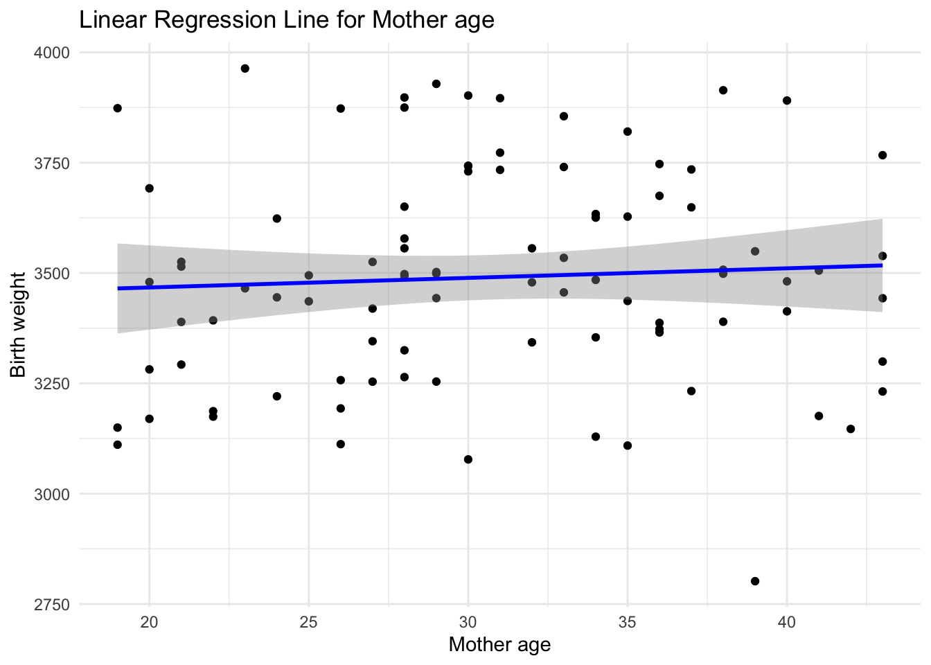
The R-squared value indicates that 84.45% of the variability in Birth_weight is explained by the predictors in the model. Significant predictors, such as Gestational_age and Smoking, provide insights into how these factors influence birth weight. For instance, a positive coefficient for Gestational_age suggests that longer gestation periods are associated with higher birth weights, while a negative coefficient for Smoking indicates that maternal smoking is associated with lower birth weights.
# Plot the regression line with the dataggplot(data, aes(x =`Mother age`, y = Birth_weight)) +geom_point() +geom_smooth(method ="lm", col ="blue") +labs(title ="Linear Regression Line for Mother age",x ="Mother age",y ="Birth weight") +theme_minimal()
`geom_smooth()` using formula = 'y ~ x'
# Repeat for other variables...
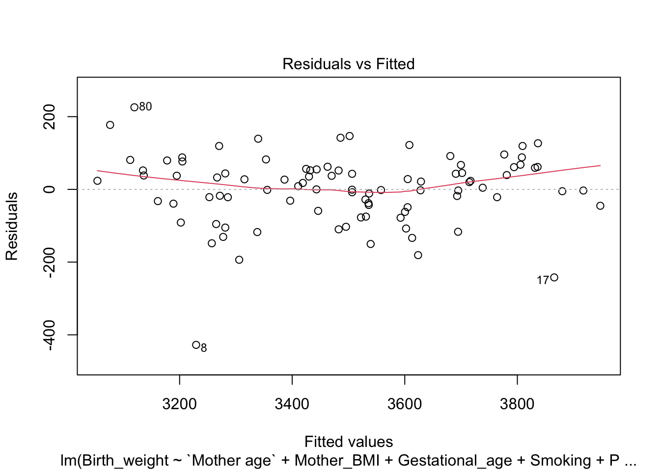
Residual vs Fitted Plot
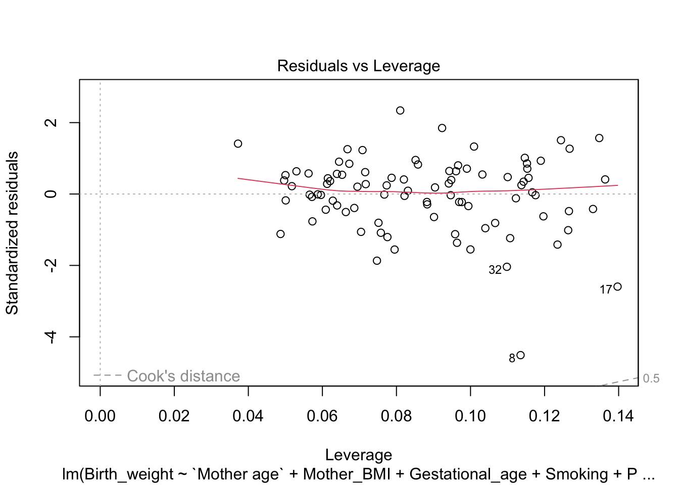
This plot shows the residuals on the y-axis and leverage on the x-axis. Leverage indicates how far away the independent variable values of an observation are from those of the other observations. High leverage points have more influence on the model’s coefficients.
plot(model, which=1)
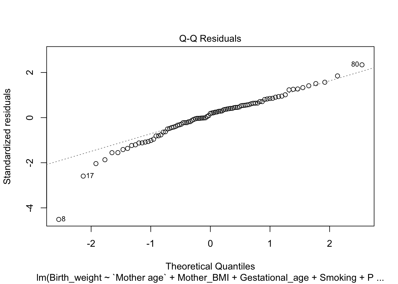
Normal Q-Q Plot
The Q-Q (Quantile-Quantile) plot compares the distribution of the residuals to a theoretical normal distribution. It plots the quantiles of the residuals against the quantiles of a standard normal distribution.
plot(model, which=2)
Warning: not plotting observations with leverage one:
  72
Model Diagnostics
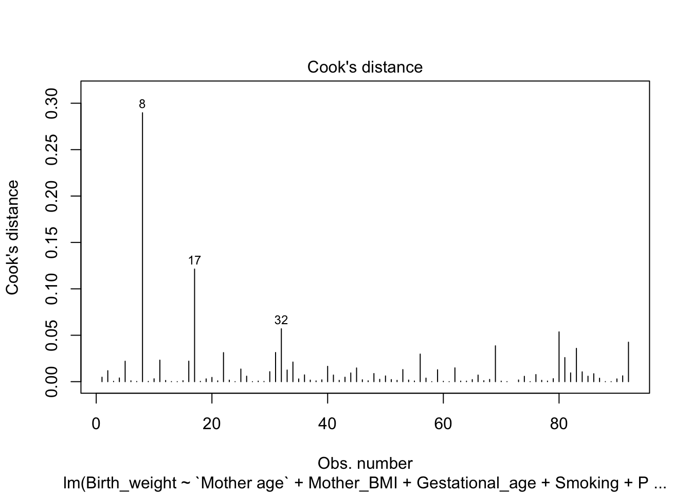
Cook’s Distance
Cook’s distance is a measure used to identify influential data points. It combines information on both leverage and residuals to indicate observations that are affecting the model fit.
plot(model, which=4)
Leverage Plot
This plot identifies points with high leverage.
plot(model, which=5)
Warning: not plotting observations with leverage one:
  72
# Summary of assumptions checksassumptions <-list("Linearity"="Checked with scatter plots","Normality"="Checked with Q-Q plot of residuals","Homoscedasticity"="Checked with Residuals vs Fitted plot","No Multicollinearity"="Checked with VIF")assumptions
$Linearity
[1] "Checked with scatter plots"

$Normality
[1] "Checked with Q-Q plot of residuals"

$Homoscedasticity
[1] "Checked with Residuals vs Fitted plot"

$`No Multicollinearity`
[1] "Checked with VIF"
10. Save the Results (Optional)
# Save the model summary to a text filecapture.output(summary(model), file ="model_summary.txt")