num <- 2.2
class(num)
## [1] "numeric"

char <- "hello"
class(char)
## [1] "character"

logi <- TRUE
class(logi)
## [1] "logical"Data in R
Until now, you’ve created fairly simple data in R and stored it as a vector. However, most (if not all) of you will have much more complicated datasets from your various experiments and surveys that go well beyond what a vector can handle. Learning how R deals with different types of data and data structures, how to import your data into R and how to manipulate and summarise your data are some of the most important skills you will need to master.
In this Chapter we’ll go over the main data types in R and focus on some of the most common data structures. We will also cover how to import data into R from an external file, how to manipulate (wrangle) and summarise data and finally how to export data from R to an external file.
Data types
Understanding the different types of data and how R deals with these data is important. The temptation is to glaze over and skip these technical details, but beware, this can come back to bite you somewhere unpleasant if you don’t pay attention. We’ve already seen an example of this when we tried (and failed) to add two character objects together using the + operator.
R has six basic types of data; numeric, integer, logical, complex and character. The keen eyed among you will notice we’ve only listed five data types here, the final data type is raw which we won’t cover as it’s not useful 99.99% of the time. We also won’t cover complex numbers as we don’t have the [imagination][complex_num]!
Numeric data are numbers that contain a decimal. Actually they can also be whole numbers but we’ll gloss over that.
Integers are whole numbers (those numbers without a decimal point).
Logical data take on the value of either
TRUEorFALSE. There’s also another special type of logical calledNAto represent missing values.Character data are used to represent string values. You can think of character strings as something like a word (or multiple words). A special type of character string is a factor, which is a string but with additional attributes (like levels or an order). We’ll cover factors later.
R is (usually) able to automatically distinguish between different classes of data by their nature and the context in which they’re used although you should bear in mind that R can’t actually read your mind and you may have to explicitly tell R how you want to treat a data type. You can find out the type (or class) of any object using the class() function.
Alternatively, you can ask if an object is a specific class using using a logical test. The is.[classOfData]() family of functions will return either a TRUE or a FALSE.
is.numeric(num)
## [1] TRUE

is.character(num)
## [1] FALSE

is.character(char)
## [1] TRUE

is.logical(logi)
## [1] TRUE
It can sometimes be useful to be able to change the class of a variable using the as.[className]() family of coercion functions, although you need to be careful when doing this as you might receive some unexpected results (see what happens below when we try to convert a character string to a numeric).
# coerce numeric to character
class(num)
## [1] "numeric"
num_char <-  as.character(num)
num_char
## [1] "2.2"
class(num_char)
## [1] "character"

# coerce character to numeric!
class(char)
## [1] "character"
char_num <- as.numeric(char)
## Warning: NAs introduced by coercion
Here’s a summary table of some of the logical test and coercion functions available to you.
| Type | Logical test | Coercing |
|---|---|---|
| Character | is.character |
as.character |
| Numeric | is.numeric |
as.numeric |
| Logical | is.logical |
as.logical |
| Factor | is.factor |
as.factor |
| Complex | is.complex |
as.complex |
Data structures
Now that you’ve been introduced to some of the most important classes of data in R, let’s have a look at some of main structures that we have for storing these data.
Scalars and vectors
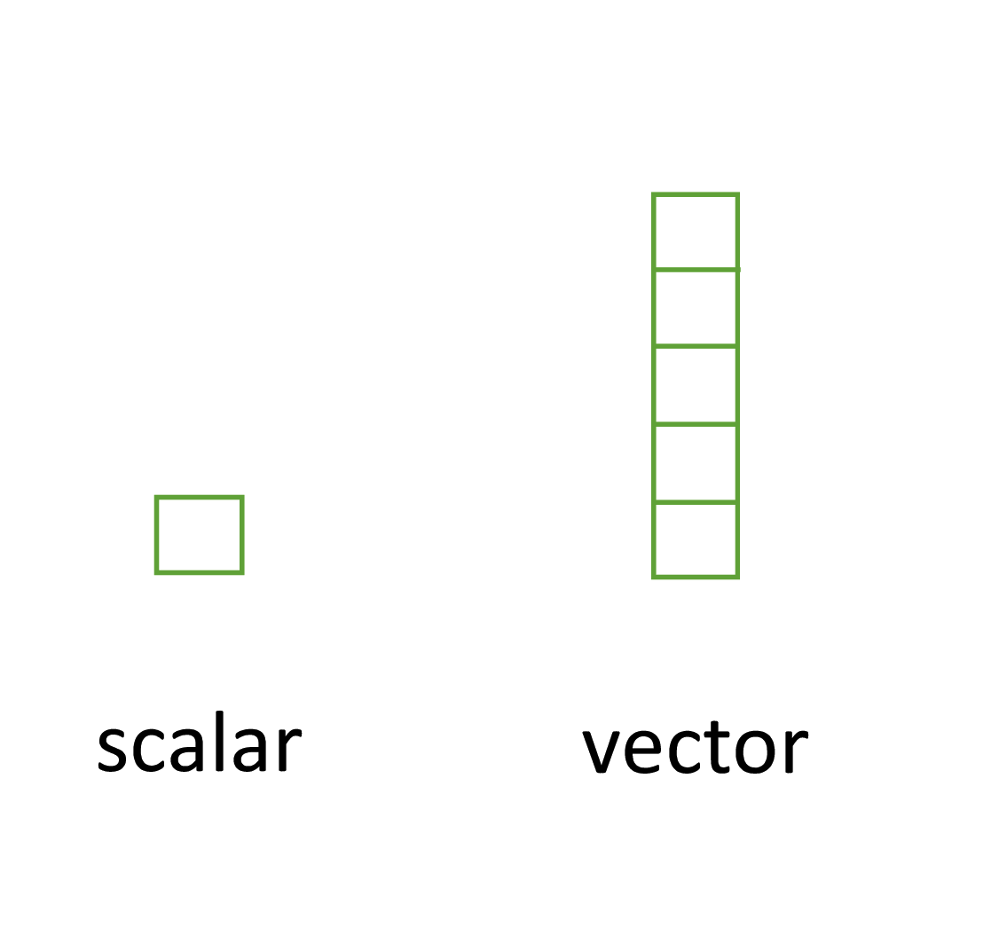
Perhaps the simplest type of data structure is the vector. You’ve already been introduced to vectors in R basics although some of the vectors you created only contained a single value. Vectors that have a single value (length 1) are called scalars. Vectors can contain numbers, characters, factors or logicals, but the key thing to remember is that all the elements inside a vector must be of the same class. In other words, vectors can contain either numbers, characters or logicals but not mixtures of these types of data. There is one important exception to this, you can include NA (remember this is special type of logical) to denote missing data in vectors with other data types.
Matrices and arrays
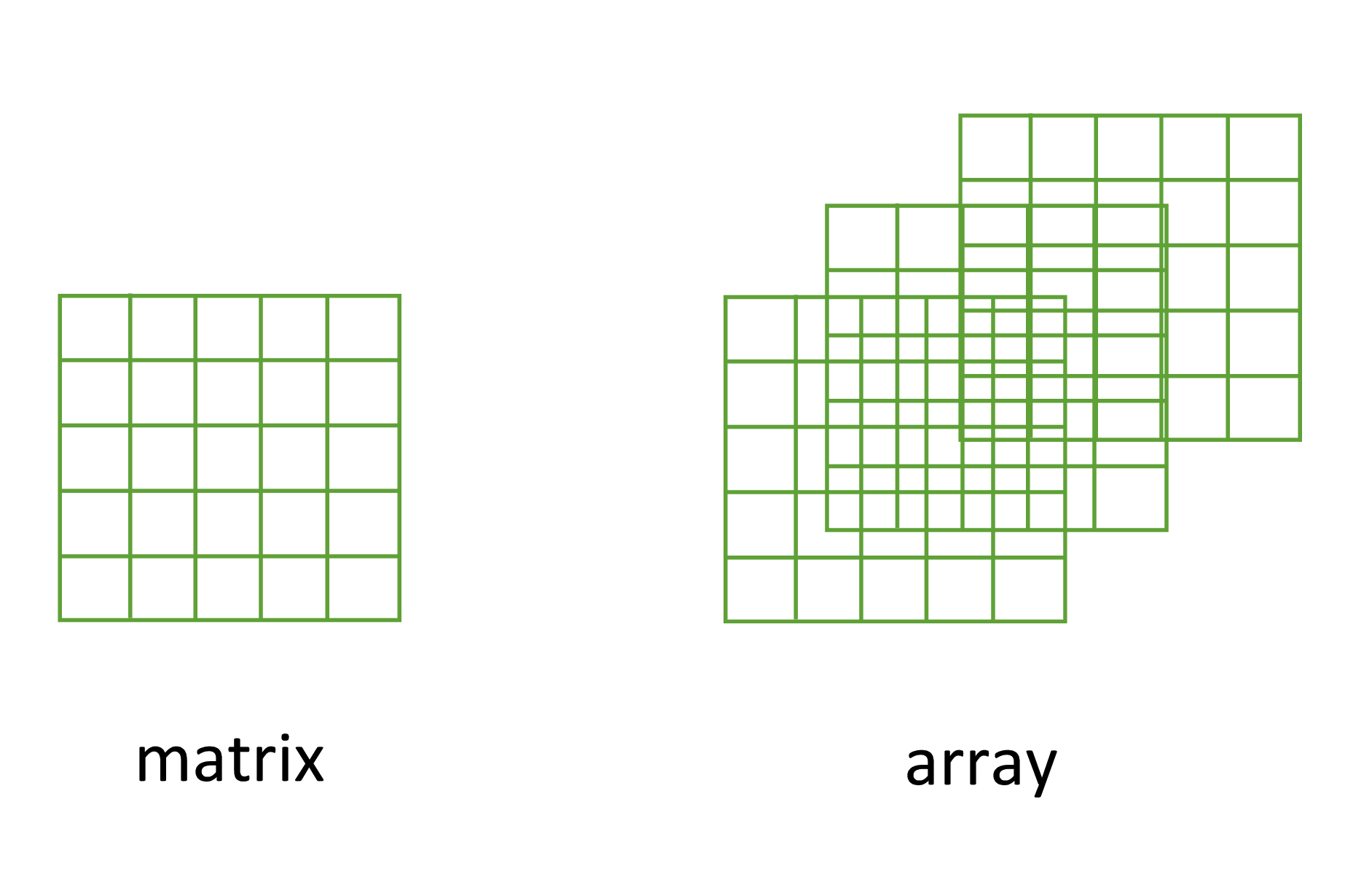
Another useful data structure used in many disciplines such as population ecology, theoretical and applied statistics is the matrix. A matrix is simply a vector that has additional attributes called dimensions. Arrays are just multidimensional matrices. Again, matrices and arrays must contain elements all of the same data class.
A convenient way to create a matrix or an array is to use the matrix() and array() functions respectively. Below, we will create a matrix from a sequence 1 to 16 in four rows (nrow = 4) and fill the matrix row-wise (byrow = TRUE) rather than the default column-wise. When using the array() function we define the dimensions using the dim = argument, in our case 2 rows, 4 columns in 2 different matrices.
my_mat <- matrix(1:16, nrow = 4, byrow = TRUE)
my_mat
##      [,1] [,2] [,3] [,4]
## [1,]    1    2    3    4
## [2,]    5    6    7    8
## [3,]    9   10   11   12
## [4,]   13   14   15   16

my_array <- array(1:16, dim = c(2, 4, 2))
my_array
## , , 1
##
##      [,1] [,2] [,3] [,4]
## [1,]    1    3    5    7
## [2,]    2    4    6    8
##
## , , 2
##
##      [,1] [,2] [,3] [,4]
## [1,]    9   11   13   15
## [2,]   10   12   14   16
Sometimes it’s also useful to define row and column names for your matrix but this is not a requirement. To do this use the rownames() and colnames() functions.
rownames(my_mat) <- c("A", "B", "C", "D")
colnames(my_mat) <- c("a", "b", "c", "d")
my_mat
##    a  b  c  d
## A  1  2  3  4
## B  5  6  7  8
## C  9 10 11 12
## D 13 14 15 16
Once you’ve created your matrices you can do useful stuff with them and as you’d expect, R has numerous built in functions to perform matrix operations. Some of the most common are given below. For example, to transpose a matrix we use the transposition function t().
my_mat_t <- t(my_mat)
my_mat_t
##   A B  C  D
## a 1 5  9 13
## b 2 6 10 14
## c 3 7 11 15
## d 4 8 12 16
To extract the diagonal elements of a matrix and store them as a vector we can use the diag() function.
my_mat_diag <- diag(my_mat)
my_mat_diag
## [1]  1  6 11 16
The usual matrix addition, multiplication etc can be performed. Note the use of the %*% operator to perform matrix multiplication.
mat.1 <- matrix(c(2, 0, 1, 1), nrow = 2)    # notice that the matrix has been filled
mat.1                                     # column-wise by default
##      [,1] [,2]
## [1,]    2    1
## [2,]    0    1

mat.2 <- matrix(c(1, 1, 0, 2), nrow = 2)
mat.2
##      [,1] [,2]
## [1,]    1    0
## [2,]    1    2

mat.1 + mat.2           # matrix addition
##      [,1] [,2]
## [1,]    3    1
## [2,]    1    3
mat.1 * mat.2           # element by element products
##      [,1] [,2]
## [1,]    2    0
## [2,]    0    2
mat.1 %*% mat.2         # matrix multiplication
##      [,1] [,2]
## [1,]    3    2
## [2,]    1    2
Lists
The next data structure we will quickly take a look at is a list. Whilst vectors and matrices are constrained to contain data of the same type, lists are able to store mixtures of data types. In fact we can even store other data structures such as vectors and arrays within a list or even have a list of a list. This makes for a very flexible data structure which is ideal for storing irregular or non-rectangular data in programming chapter for an example).
To create a list we can use the list() function. Note how each of the three list elements are of different classes (character, logical, and numeric) and are of different lengths.
list_1 <- list(c("black", "yellow", "orange"),
               c(TRUE, TRUE, FALSE, TRUE, FALSE, FALSE),
               matrix(1:6, nrow = 3))
list_1
## [[1]]
## [1] "black"  "yellow" "orange"
##
## [[2]]
## [1]  TRUE  TRUE FALSE  TRUE FALSE FALSE
##
## [[3]]
##      [,1] [,2]
## [1,]    1    4
## [2,]    2    5
## [3,]    3    6
Elements of the list can be named during the construction of the list
list_2 <- list(colours = c("black", "yellow", "orange"),
               evaluation = c(TRUE, TRUE, FALSE, TRUE, FALSE, FALSE),
               time = matrix(1:6, nrow = 3))
list_2
## $colours
## [1] "black"  "yellow" "orange"
##
## $evaluation
## [1]  TRUE  TRUE FALSE  TRUE FALSE FALSE
##
## $time
##      [,1] [,2]
## [1,]    1    4
## [2,]    2    5
## [3,]    3    6
or after the list has been created using the names() function.
names(list_1) <- c("colours", "evaluation", "time")
list_1
## $colours
## [1] "black"  "yellow" "orange"
##
## $evaluation
## [1]  TRUE  TRUE FALSE  TRUE FALSE FALSE
##
## $time
##      [,1] [,2]
## [1,]    1    4
## [2,]    2    5
## [3,]    3    6
Data frames
Take a look at this [video][dataf-vid] for a quick introduction to data frame objects in R
By far the most commonly used data structure to store data in is the data frame. A data frame is a powerful two-dimensional object made up of rows and columns which looks superficially very similar to a matrix. However, whilst matrices are restricted to containing data all of the same type, data frames can contain a mixture of different types of data. Typically, in a data frame each row corresponds to an individual observation and each column corresponds to a different measured or recorded variable. This setup may be familiar to those of you who use LibreOffice Calc or Microsoft Excel to manage and store your data. Perhaps a useful way to think about data frames is that they are essentially made up of a bunch of vectors (columns) with each vector containing its own data type but the data type can be different between vectors.
As an example, the data frame below contains the results of an experiment to determine the effect of removing the tip of petunia plants (Petunia sp.) grown at 3 levels of nitrogen on various measures of growth (note: data shown below are a subset of the full dataset). The data frame has 8 variables (columns) and each row represents an individual plant. The variables treat and nitrogen are factors ([categorical][cat-var] variables). The treat variable has 2 levels (tip and notip) and the nitrogen level variable has 3 levels (low, medium and high). The variables height, weight, leafarea and shootarea are numeric and the variable flowers is an integer representing the number of flowers. Although the variable block has numeric values, these do not really have any order and could also be treated as a factor (i.e. they could also have been called A and B).
| treat | nitrogen | block | height | weight | leafarea | shootarea | flowers |
|---|---|---|---|---|---|---|---|
| tip | medium | 1 | 7.5 | 7.62 | 11.7 | 31.9 | 1 |
| tip | medium | 1 | 10.7 | 12.14 | 14.1 | 46.0 | 10 |
| tip | medium | 1 | 11.2 | 12.76 | 7.1 | 66.7 | 10 |
| tip | medium | 1 | 10.4 | 8.78 | 11.9 | 20.3 | 1 |
| tip | medium | 1 | 10.4 | 13.58 | 14.5 | 26.9 | 4 |
| tip | medium | 1 | 9.8 | 10.08 | 12.2 | 72.7 | 9 |
| notip | low | 2 | 3.7 | 8.10 | 10.5 | 60.5 | 6 |
| notip | low | 2 | 3.2 | 7.45 | 14.1 | 38.1 | 4 |
| notip | low | 2 | 3.9 | 9.19 | 12.4 | 52.6 | 9 |
| notip | low | 2 | 3.3 | 8.92 | 11.6 | 55.2 | 6 |
| notip | low | 2 | 5.5 | 8.44 | 13.5 | 77.6 | 9 |
| notip | low | 2 | 4.4 | 10.60 | 16.2 | 63.3 | 6 |
There are a couple of important things to bear in mind about data frames. These types of objects are known as rectangular data (or tidy data) as each column must have the same number of observations. Also, any missing data should be recorded as an NA just as we did with our vectors.
We can construct a data frame from existing data objects such as vectors using the data.frame() function. As an example, let’s create three vectors p.height, p.weight and p.names and include all of these vectors in a data frame object called dataf.
p.height <- c(180, 155, 160, 167, 181)
p.weight <- c(65, 50, 52, 58, 70)
p.names <- c("Joanna", "Charlotte", "Helen", "Karen", "Amy")

dataf <- data.frame(height = p.height, weight = p.weight, names = p.names)
dataf
##   height weight     names
## 1    180     65    Joanna
## 2    155     50 Charlotte
## 3    160     52     Helen
## 4    167     58     Karen
## 5    181     70       Amy
You’ll notice that each of the columns are named with variable name we supplied when we used the data.frame() function. It also looks like the first column of the data frame is a series of numbers from one to five. Actually, this is not really a column but the name of each row. We can check this out by getting R to return the dimensions of the dataf object using the dim() function. We see that there are 5 rows and 3 columns.
dim(dataf)   # 5 rows and 3 columns
## [1] 5 3
Another really useful function which we use all the time is str() which will return a compact summary of the structure of the data frame object (or any object for that matter).
str(dataf)
## 'data.frame':    5 obs. of  3 variables:
##  $ height: num  180 155 160 167 181
##  $ weight: num  65 50 52 58 70
##  $ names : chr  "Joanna" "Charlotte" "Helen" "Karen" ...
The str() function gives us the data frame dimensions and also reminds us that dataf is a data.frame type object. It also lists all of the variables (columns) contained in the data frame, tells us what type of data the variables contain and prints out the first five values. We often copy this summary and place it in our R scripts with comments at the beginning of each line so we can easily refer back to it whilst writing our code. We showed you how to comment blocks in RStudio here.
Also notice that R has automatically decided that our p.names variable should be a character (chr) class variable when we first created the data frame. Whether this is a good idea or not will depend on how you want to use this variable in later analysis. If we decide that this wasn’t such a good idea we can change the default behaviour of the data.frame() function by including the argument stringsAsFactors = TRUE. Now our strings are automatically converted to factors.
p.height <- c(180, 155, 160, 167, 181)
p.weight <- c(65, 50, 52, 58, 70)
p.names <- c("Joanna", "Charlotte", "Helen", "Karen", "Amy")

dataf <- data.frame(height = p.height, weight = p.weight, names = p.names,
                                        stringsAsFactors = TRUE)
str(dataf)
## 'data.frame':    5 obs. of  3 variables:
##  $ height: num  180 155 160 167 181
##  $ weight: num  65 50 52 58 70
##  $ names : Factor w/ 5 levels "Amy","Charlotte",..: 4 2 3 5 1
Importing data
Although creating data frames from existing data structures is extremely useful, by far the most common approach is to create a data frame by importing data from an external file. To do this, you’ll need to have your data correctly formatted and saved in a file format that R is able to recognise. Fortunately for us, R is able to recognise a wide variety of file formats, although in reality you’ll probably end up only using two or three regularly.
Take a look at this [video][import-vid] for a quick introduction to importing data in R
Saving files to import
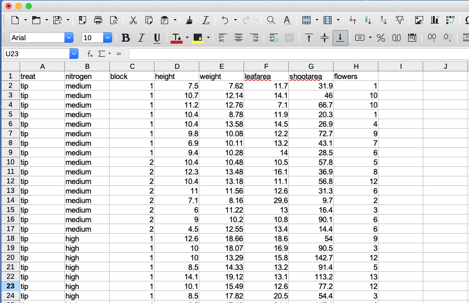
The easiest method of creating a data file to import into R is to enter your data into a spreadsheet using either Microsoft Excel or LibreOffice Calc and save the spreadsheet as a tab delimited file. We prefer LibreOffice Calc as it’s open source, platform independent and free but MS Excel is OK too (but see [here][excel_gotcha] for some gotchas). Here’s the data from the petunia experiment we dicussed previously displayed in LibreOffice. If you want to follow along you can download the data file (‘flower.xls’) from the companion website [here][flow-data].
For those of you unfamiliar with the tab delimited file format it simply means that data in different columns are separated with a ‘tab’ character (yes, the same one as on your keyboard) and is usually saved as a file with a ‘.txt’ extension (you might also see .tsv which is short for tab separated values).
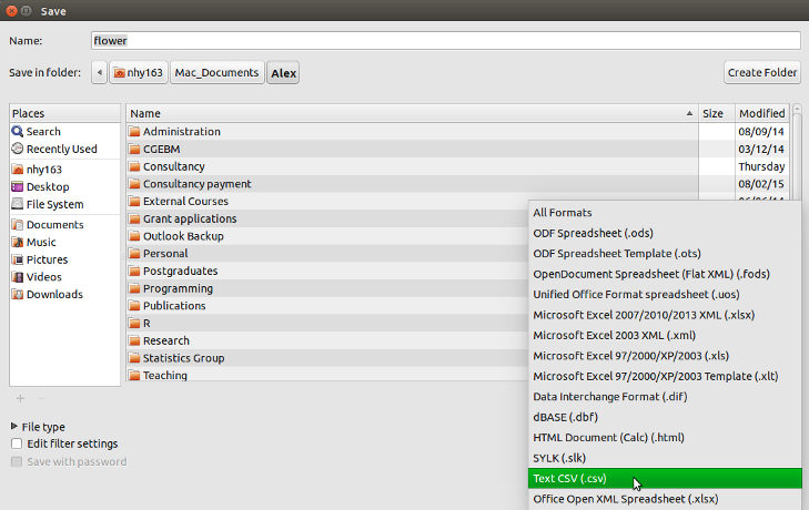
To save a spreadsheet as a tab delimited file in LibreOffice Calc select File -> Save as ... from the main menu. You will need to specify the location you want to save your file in the ‘Save in folder’ option and the name of the file in the ‘Name’ option. In the drop down menu located above the ‘Save’ button change the default ‘All formats’ to ‘Text CSV (.csv)’.
Click the Save button and then select the ‘Use Text CSV Format’ option. In the next pop-up window select {Tab} from the drop down menu in the ‘Field delimiter’ option. Click on OK to save the file.
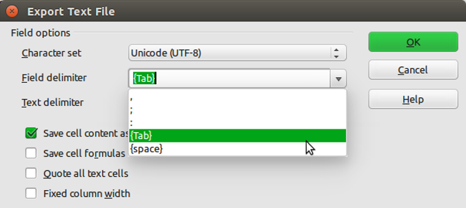
The resulting file will annoyingly have a ‘.csv’ extension even though we’ve saved it as a tab delimited file. Either live with it or rename the file with a ‘.txt’ extension instead.
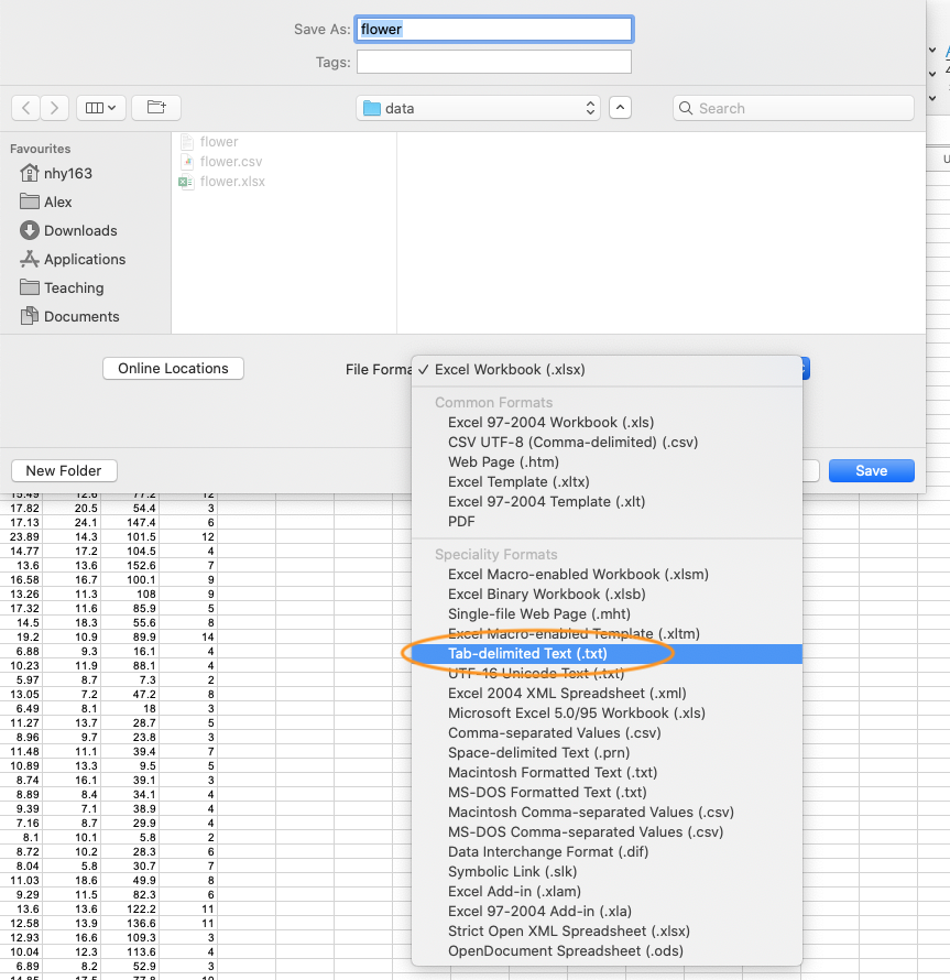
In MS Excel, select File -> Save as ... from the main menu and navigate to the folder where you want to save the file. Enter the file name (keep it fairly short, no spaces!) in the ‘Save as:’ dialogue box. In the ‘File format:’ dialogue box click on the down arrow to open the drop down menu and select ‘Text (Tab delimited)’ as your file type. Select OK to save the file.
There are a couple of things to bear in mind when saving files to import into R which will make your life easier in the long run. Keep your column headings (if you have them) short and informative. Also avoid spaces in your column headings by replacing them with an underscore or a dot (i.e. replace shoot height with shoot_height or shoot.height) and avoid using special characters (i.e. leaf area (mm^2)). Remember, if you have missing data in your data frame (empty cells) you should use an NA to represent these missing values. This will keep the data frame tidy.
Import functions
Once you’ve saved your data file in a suitable format we can now read this file into R. The workhorse function for importing data into R is the read.table() function (we discuss some alternatives later in the chapter). The read.table() function is a very flexible function with a shed load of arguments (see ?read.table) but it’s quite simple to use. Let’s import a tab delimited file called flower.txt which contains the data assign it to an object called flowers. The file is located in a data directory which itself is located in our root directory. The first row of the data contains the variable (column) names. To use the read.table() function to import this file.
flowers <- read.table(file = 'data/flower.txt', header = TRUE, sep = "\t",
                        stringsAsFactors = TRUE)
There are a few things to note about the above command. First, the file path and the filename (including the file extension) needs to be enclosed in either single or double quotes (i.e. the data/flower.txt bit) as the read.table() function expects this to be a character string. If your working directory is already set to the directory which contains the file, you don’t need to include the entire file path just the filename. In the example above, the file path is separated with a single forward slash /. This will work regardless of the operating system you are using and we recommend you stick with this. However, Windows users may be more familiar with the single backslash notation and if you want to keep using this you will need to include them as double backslashes. Note though that the double backslash notation will not work on computers using Mac OSX or Linux operating systems.
flowers <- read.table(file = 'C:\\Documents\\Prog1\\data\\flower.txt',
                      header = TRUE, sep = "\t", stringsAsFactors = TRUE)
The header = TRUE argument specifies that the first row of your data contains the variable names (i.e. nitrogen, block etc). If this is not the case you can specify header = FALSE (actually, this is the default value so you can omit this argument entirely). The sep = "\t" argument tells R that the file delimiter is a tab (\t).
After importing our data into R it doesn’t appear that R has done much, at least nothing appears in the R Console! To see the contents of the data frame we could just type the name of the object as we have done previously. BUT before you do that, think about why you’re doing this. If your data frame is anything other than tiny, all you’re going to do is fill up your Console with data. It’s not like you can easily check whether there are any errors or that your data has been imported correctly. A much better solution is to use our old friend the str() function to return a compact and informative summary of your data frame.
str(flowers)
## 'data.frame':    96 obs. of  8 variables:
##  $ treat    : Factor w/ 2 levels "notip","tip": 2 2 2 2 2 2 2 2 2 2 ...
##  $ nitrogen : Factor w/ 3 levels "high","low","medium": 3 3 3 3 3 3 3 3 3 3 ...
##  $ block    : int  1 1 1 1 1 1 1 1 2 2 ...
##  $ height   : num  7.5 10.7 11.2 10.4 10.4 9.8 6.9 9.4 10.4 12.3 ...
##  $ weight   : num  7.62 12.14 12.76 8.78 13.58 ...
##  $ leafarea : num  11.7 14.1 7.1 11.9 14.5 12.2 13.2 14 10.5 16.1 ...
##  $ shootarea: num  31.9 46 66.7 20.3 26.9 72.7 43.1 28.5 57.8 36.9 ...
##  $ flowers  : int  1 10 10 1 4 9 7 6 5 8 ...
Here we see that flowers is a ‘data.frame’ object which contains 96 rows and 8 variables (columns). Each of the variables are listed along with their data class and the first 10 values. As we mentioned previously in this Chapter, it can be quite convenient to copy and paste this into your R script as a comment block for later reference.
Notice also that your character string variables (treat and nitrogen) have been imported as factors because we used the argument stringsAsFactors = TRUE. If this is not what you want you can prevent this by using the stringsAsFactors = FALSE or from R version 4.0.0 you can just leave out this argument as stringsAsFactors = FALSE is the default.
flowers <- read.table(file = 'data/flower.txt', header = TRUE,
                      sep = "\t", stringsAsFactors = FALSE)
str(flowers)
## 'data.frame':    96 obs. of  8 variables:
##  $ treat    : chr  "tip" "tip" "tip" "tip" ...
##  $ nitrogen : chr  "medium" "medium" "medium" "medium" ...
##  $ block    : int  1 1 1 1 1 1 1 1 2 2 ...
##  $ height   : num  7.5 10.7 11.2 10.4 10.4 9.8 6.9 9.4 10.4 12.3 ...
##  $ weight   : num  7.62 12.14 12.76 8.78 13.58 ...
##  $ leafarea : num  11.7 14.1 7.1 11.9 14.5 12.2 13.2 14 10.5 16.1 ...
##  $ shootarea: num  31.9 46 66.7 20.3 26.9 72.7 43.1 28.5 57.8 36.9 ...
##  $ flowers  : int  1 10 10 1 4 9 7 6 5 8 ...
Other useful arguments include dec = and na.strings =. The dec = argument allows you to change the default character (.) used for a decimal point. This is useful if you’re in a country where decimal places are usually represented by a comma (i.e. dec = ","). The na.strings = argument allows you to import data where missing values are represented with a symbol other than NA. This can be quite common if you are importing data from other statistical software such as Minitab which represents missing values as a * (na.strings = "*").
If we just wanted to see the names of our variables (columns) in the data frame we can use the names() function which will return a character vector of the variable names.
names(flowers)
## [1] "treat"     "nitrogen"  "block"     "height"    "weight"    "leafarea"
## [7] "shootarea" "flowers"
R has a number of variants of the read.table() function that you can use to import a variety of file formats. Actually, these variants just use the read.table() function but include different combinations of arguments by default to help import different file types. The most useful of these are the read.csv(), read.csv2() and read.delim() functions. The read.csv() function is used to import comma separated value (.csv) files and assumes that the data in columns are separated by a comma (it sets sep = "," by default). It also assumes that the first row of the data contains the variable names by default (it sets header = TRUE by default). The read.csv2() function assumes data are separated by semicolons and that a comma is used instead of a decimal point (as in many European countries). The read.delim() function is used to import tab delimited data and also assumes that the first row of the data contains the variable names by default.
# import .csv file
flowers <- read.csv(file = 'data/flower.csv')

# import .csv file with dec = "," and sep = ";"
flowers <- read.csv2(file = 'data/flower.csv')

# import tab delim file with sep = "\t"
flowers <- read.delim(file = 'data/flower.txt')
You can even import spreadsheet files from MS Excel or other statistics software directly into R but our advice is that this should generally be avoided if possible as it just adds a layer of uncertainty between you and your data. In our opinion it’s almost always better to export your spreadsheets as tab or comma delimited files and then import them into R using the read.table() function. If you’re hell bent on directly importing data from other software you will need to install the foreign package which has functions for importing Minitab, SPSS, Stata and SAS files or the xlsx package to import Excel spreadsheets.
Common import frustrations
It’s quite common to get a bunch of really frustrating error messages when you first start importing data into R. Perhaps the most common is
Error in file(file, "rt") : cannot open the connection
In addition: Warning message:
In file(file, "rt") :
  cannot open file 'flower.txt': No such file or directory
This error message is telling you that R cannot find the file you are trying to import. It usually rears its head for one of a couple of reasons (or all of them!). The first is that you’ve made a mistake in the spelling of either the filename or file path. Another common mistake is that you have forgotten to include the file extension in the filename (i.e. .txt). Lastly, the file is not where you say it is or you’ve used an incorrect file path. Using RStudio Projects and having a logical directory structure goes a long way to avoiding these types of errors.
Another really common mistake is to forget to include the header = TRUE argument when the first row of the data contains variable names. For example, if we omit this argument when we import our flowers.txt file everything looks OK at first (no error message at least)
flowers_bad <- read.table(file = 'data/flower.txt', sep = "\t")but when we take a look at our data frame using str()
str(flowers_bad)
## 'data.frame':    97 obs. of  8 variables:
##  $ V1: chr  "treat" "tip" "tip" "tip" ...
##  $ V2: chr  "nitrogen" "medium" "medium" "medium" ...
##  $ V3: chr  "block" "1" "1" "1" ...
##  $ V4: chr  "height" "7.5" "10.7" "11.2" ...
##  $ V5: chr  "weight" "7.62" "12.14" "12.76" ...
##  $ V6: chr  "leafarea" "11.7" "14.1" "7.1" ...
##  $ V7: chr  "shootarea" "31.9" "46" "66.7" ...
##  $ V8: chr  "flowers" "1" "10" "10" ...
We can see an obvious problem, all of our variables have been imported as factors and our variables are named V1, V2, V3 … V8. The problem happens because we haven’t told the read.table() function that the first row contains the variable names and so it treats them as data. As soon as we have a single character string in any of our data vectors, R treats the vectors as character type data (remember all elements in a vector must contain the same type of data).
Other import options
There are numerous other functions to import data from a variety of sources and formats. Most of these functions are contained in packages that you will need to install before using them. We list a couple of the more useful packages and functions below.
The fread() function from the data.table package is great for importing large data files quickly and efficiently (much faster than the read.table() function). One of the great things about the fread() function is that it will automatically detect many of the arguments you would normally need to specify (like sep = etc). One thing you might need to consider is that the fread() function will return a data.table object by default not a data.frame as would be the case with the read.table() function. This is usually not a problem and you can change this default behaviour by using the argument data.table = FALSE when you use fread() if you prefer a data.frame object. To learn more about the differences between data.table and data.frame objects see [here][data-table].
library(data.table)
all_data <- fread(file = 'data/flower.txt')
Various functions from the readr package are also very efficient at reading in large data files. The readr package is part of the ‘[tidyverse][tidyverse]’ collection of packages and provides many equivalent functions to base R for importing data. The readr functions are used in a similar way to the read.table() or read.csv() functions and many of the arguments are the same (see ?readr::read_table for more details). There are however some differences. For example, when using the read_table() function the header = TRUE argument is replaced by col_names = TRUE and the function returns a tibble class object which is the tidyverse equivalent of a data.frame object (see [here][tibbles] for differences).
library(readr)
# import white space delimited files
all_data <- read_table(file = 'data/flower.txt', col_names = TRUE)

# import comma delimited files
all_data <- read_csv(file = 'data/flower.txt')

# import tab delimited files
all_data <- read_delim(file = 'data/flower.txt', delim = "\t")

# or use
all_data <- read_tsv(file = 'data/flower.txt')
If your data file is ginormous, then the ff and bigmemory packages may be useful as they both contain import functions that are able to store large data in a memory efficient manner. You can find out more about these functions [here][ff] and [here][bigmem].
Wrangling data frames
Now that you’re able to successfully import your data from an external file into R our next task is to do something useful with our data. Working with data is a fundamental skill which you’ll need to develop and get comfortable with as you’ll likely do a lot of it during any project. The good news is that R is especially good at manipulating, summarising and visualising data. Manipulating data (often known as data wrangling or munging) in R can at first seem a little daunting for the new user but if you follow a few simple logical rules then you’ll quickly get the hang of it, especially with some practice.
See this [video][dataw-vid] for a general overview on how to use positional and logical indexes to extract data from a data frame object in R
Let’s remind ourselves of the structure of the flowers data frame we imported in the previous section.
flowers <- read.table(file = 'data/flower.txt', header = TRUE, sep = "\t")
str(flowers)
## 'data.frame':    96 obs. of  8 variables:
##  $ treat    : chr  "tip" "tip" "tip" "tip" ...
##  $ nitrogen : chr  "medium" "medium" "medium" "medium" ...
##  $ block    : int  1 1 1 1 1 1 1 1 2 2 ...
##  $ height   : num  7.5 10.7 11.2 10.4 10.4 9.8 6.9 9.4 10.4 12.3 ...
##  $ weight   : num  7.62 12.14 12.76 8.78 13.58 ...
##  $ leafarea : num  11.7 14.1 7.1 11.9 14.5 12.2 13.2 14 10.5 16.1 ...
##  $ shootarea: num  31.9 46 66.7 20.3 26.9 72.7 43.1 28.5 57.8 36.9 ...
##  $ flowers  : int  1 10 10 1 4 9 7 6 5 8 ...
To access the data in any of the variables (columns) in our data frame we can use the $ notation. For example, to access the height variable in our flowers data frame we can use flowers$height. This tells R that the height variable is contained within the data frame flowers.
flowers$height
##  [1]  7.5 10.7 11.2 10.4 10.4  9.8  6.9  9.4 10.4 12.3 10.4 11.0  7.1  6.0  9.0
## [16]  4.5 12.6 10.0 10.0  8.5 14.1 10.1  8.5  6.5 11.5  7.7  6.4  8.8  9.2  6.2
## [31]  6.3 17.2  8.0  8.0  6.4  7.6  9.7 12.3  9.1  8.9  7.4  3.1  7.9  8.8  8.5
## [46]  5.6 11.5  5.8  5.6  5.3  7.5  4.1  3.5  8.5  4.9  2.5  5.4  3.9  5.8  4.5
## [61]  8.0  1.8  2.2  3.9  8.5  8.5  6.4  1.2  2.6 10.9  7.2  2.1  4.7  5.0  6.5
## [76]  2.6  6.0  9.3  4.6  5.2  3.9  2.3  5.2  2.2  4.5  1.8  3.0  3.7  2.4  5.7
## [91]  3.7  3.2  3.9  3.3  5.5  4.4
This will return a vector of the height data. If we want we can assign this vector to another object and do stuff with it, like calculate a mean or get a summary of the variable using the summary() function.
f_height <- flowers$height
mean(f_height)
## [1] 6.839583
summary(f_height)
##    Min. 1st Qu.  Median    Mean 3rd Qu.    Max.
##   1.200   4.475   6.450   6.840   9.025  17.200
Or if we don’t want to create an additional object we can use functions ‘on-the-fly’ to only display the value in the console.
mean(flowers$height)
## [1] 6.839583
summary(flowers$height)
##    Min. 1st Qu.  Median    Mean 3rd Qu.    Max.
##   1.200   4.475   6.450   6.840   9.025  17.200
Just as we did with vectors, we also can access data in data frames using the square bracket [ ] notation. However, instead of just using a single index, we now need to use two indexes, one to specify the rows and one for the columns. To do this, we can use the notation my_data[rows, columns] where rows and columns are indexes and my_data is the name of the data frame. Again, just like with our vectors our indexes can be positional or the result of a logical test.
Positional indexes
To use positional indexes we simple have to write the position of the rows and columns we want to extract inside the [ ]. For example, if for some reason we wanted to extract the first value (1st row ) of the height variable (4th column).
flowers[1, 4]
## [1] 7.5

# this would give you the same
flowers$height[1]
## [1] 7.5
We can also extract values from multiple rows or columns by specifying these indexes as vectors inside the [ ]. To extract the first 10 rows and the first 4 columns we simple supply a vector containing a sequence from 1 to 10 for the rows index (1:10) and a vector from 1 to 4 for the column index (1:4).
flowers[1:10, 1:4]
##    treat nitrogen block height
## 1    tip   medium     1    7.5
## 2    tip   medium     1   10.7
## 3    tip   medium     1   11.2
## 4    tip   medium     1   10.4
## 5    tip   medium     1   10.4
## 6    tip   medium     1    9.8
## 7    tip   medium     1    6.9
## 8    tip   medium     1    9.4
## 9    tip   medium     2   10.4
## 10   tip   medium     2   12.3
Or for non sequential rows and columns then we can supply vectors of positions using the c() function. To extract the 1st, 5th, 12th, 30th rows from the 1st, 3rd, 6th and 8th columns.
flowers[c(1, 5, 12, 30), c(1, 3, 6, 8)]
##    treat block leafarea flowers
## 1    tip     1     11.7       1
## 5    tip     1     14.5       4
## 12   tip     2     12.6       6
## 30   tip     2     11.6       5
All we are doing in the two examples above is creating vectors of positions for the rows and columns that we want to extract. We have done this by using the skills we developed in functions when we generated vectors using the c() function or using the : notation.
But what if we want to extract either all of the rows or all of the columns? It would be extremely tedious to have to generate vectors for all rows or for all columns. Thankfully R has a shortcut. If you don’t specify either a row or column index in the [ ] then R interprets it to mean you want all rows or all columns. For example, to extract the first 8 rows and all of the columns in the flower data frame
flowers[1:8, ]
##   treat nitrogen block height weight leafarea shootarea flowers
## 1   tip   medium     1    7.5   7.62     11.7      31.9       1
## 2   tip   medium     1   10.7  12.14     14.1      46.0      10
## 3   tip   medium     1   11.2  12.76      7.1      66.7      10
## 4   tip   medium     1   10.4   8.78     11.9      20.3       1
## 5   tip   medium     1   10.4  13.58     14.5      26.9       4
## 6   tip   medium     1    9.8  10.08     12.2      72.7       9
## 7   tip   medium     1    6.9  10.11     13.2      43.1       7
## 8   tip   medium     1    9.4  10.28     14.0      28.5       6
or all of the rows and the first 3 columns. If you’re reading the web version of this book scroll down in output panel to see all of the data. Note, if you’re reading the pdf version of the book some of the output has been truncated to save some space.
flowers[, 1:3]## treat nitrogen block
## 1 tip medium 1
## 2 tip medium 1
## 3 tip medium 1
## 4 tip medium 1
## 5 tip medium 1
## 6 tip medium 1
## 7 tip medium 1
## 8 tip medium 1
## 9 tip medium 2
## 10 tip medium 2
## 11 tip medium 2
## 12 tip medium 2
## 13 tip medium 2
## 14 tip medium 2
## 15 tip medium 2
## 16 tip medium 2
## 17 tip high 1
## 18 tip high 1
## 19 tip high 1
## 20 tip high 1
## 21 tip high 1
## 22 tip high 1
## 23 tip high 1
## 24 tip high 1
## 25 tip high 2
## 26 tip high 2
## 27 tip high 2
## 28 tip high 2
## 29 tip high 2
## 30 tip high 2
## 31 tip high 2
## 32 tip high 2
## 33 tip low 1
## 34 tip low 1
## 35 tip low 1
## 36 tip low 1
## 37 tip low 1
## 38 tip low 1
## 39 tip low 1
## 40 tip low 1
## 41 tip low 2
## 42 tip low 2
## 43 tip low 2
## 44 tip low 2
## 45 tip low 2
## 46 tip low 2
## 47 tip low 2
## 48 tip low 2
## 49 notip medium 1
## 50 notip medium 1
## 51 notip medium 1
## 52 notip medium 1
## 53 notip medium 1
## 54 notip medium 1
## 55 notip medium 1
## 56 notip medium 1
## 57 notip medium 2
## 58 notip medium 2
## 59 notip medium 2
## 60 notip medium 2
## 61 notip medium 2
## 62 notip medium 2
## 63 notip medium 2
## 64 notip medium 2
## 65 notip high 1
## 66 notip high 1
## 67 notip high 1
## 68 notip high 1
## 69 notip high 1
## 70 notip high 1
## 71 notip high 1
## 72 notip high 1
## 73 notip high 2
## 74 notip high 2
## 75 notip high 2
## 76 notip high 2
## 77 notip high 2
## 78 notip high 2
## 79 notip high 2
## 80 notip high 2
## 81 notip low 1
## 82 notip low 1
## 83 notip low 1
## 84 notip low 1
## 85 notip low 1
## 86 notip low 1
## 87 notip low 1
## 88 notip low 1
## 89 notip low 2
## 90 notip low 2
## 91 notip low 2
## 92 notip low 2
## 93 notip low 2
## 94 notip low 2
## 95 notip low 2
## 96 notip low 2We can even use negative positional indexes to exclude certain rows and columns. As an example, lets extract all of the rows except the first 85 rows and all columns except the 4th, 7th and 8th columns. Notice we need to use -() when we generate our row positional vectors. If we had just used -1:85 this would actually generate a regular sequence from -1 to 85 which is not what we want (we can of course use -1:-85).
flowers[-(1:85), -c(4, 7, 8)]
##    treat nitrogen block weight leafarea
## 86 notip      low     1   6.01     17.6
## 87 notip      low     1   9.93     12.0
## 88 notip      low     1   7.03      7.9
## 89 notip      low     2   9.10     14.5
## 90 notip      low     2   9.05      9.6
## 91 notip      low     2   8.10     10.5
## 92 notip      low     2   7.45     14.1
## 93 notip      low     2   9.19     12.4
## 94 notip      low     2   8.92     11.6
## 95 notip      low     2   8.44     13.5
## 96 notip      low     2  10.60     16.2
In addition to using a positional index for extracting particular columns (variables) we can also name the variables directly when using the square bracket [ ] notation. For example, let’s extract the first 5 rows and the variables treat, nitrogen and leafarea. Instead of using flowers[1:5, c(1, 2, 6)] we can instead use
flowers[1:5, c("treat", "nitrogen", "leafarea")]
##   treat nitrogen leafarea
## 1   tip   medium     11.7
## 2   tip   medium     14.1
## 3   tip   medium      7.1
## 4   tip   medium     11.9
## 5   tip   medium     14.5
We often use this method in preference to the positional index for selecting columns as it will still give us what we want even if we’ve changed the order of the columns in our data frame for some reason.
Logical indexes
Just as we did with vectors, we can also extract data from our data frame based on a logical test. We can use all of the logical operators that we used for our vector examples so if these have slipped your mind maybe pop back and refresh your memory. Let’s extract all rows where height is greater than 12 and extract all columns by default (remember, if you don’t include a column index after the comma it means all columns).
big_flowers <- flowers[flowers$height > 12, ]
big_flowers
##    treat nitrogen block height weight leafarea shootarea flowers
## 10   tip   medium     2   12.3  13.48     16.1      36.9       8
## 17   tip     high     1   12.6  18.66     18.6      54.0       9
## 21   tip     high     1   14.1  19.12     13.1     113.2      13
## 32   tip     high     2   17.2  19.20     10.9      89.9      14
## 38   tip      low     1   12.3  11.27     13.7      28.7       5
Notice in the code above that we need to use the flowers$height notation for the logical test. If we just named the height variable without the name of the data frame we would receive an error telling us R couldn’t find the variable height. The reason for this is that the height variable only exists inside the flowers data frame so you need to tell R exactly where it is.
big_flowers <- flowers[height > 12, ]
Error in `[.data.frame`(flowers, height > 12, ) :
  object 'height' not found
So how does this work? The logical test is flowers$height > 12 and R will only extract those rows that satisfy this logical condition. If we look at the output of just the logical condition you can see this returns a vector containing TRUE if height is greater than 12 and FALSE if height is not greater than 12.
flowers$height > 12
##  [1] FALSE FALSE FALSE FALSE FALSE FALSE FALSE FALSE FALSE  TRUE FALSE FALSE
## [13] FALSE FALSE FALSE FALSE  TRUE FALSE FALSE FALSE  TRUE FALSE FALSE FALSE
## [25] FALSE FALSE FALSE FALSE FALSE FALSE FALSE  TRUE FALSE FALSE FALSE FALSE
## [37] FALSE  TRUE FALSE FALSE FALSE FALSE FALSE FALSE FALSE FALSE FALSE FALSE
## [49] FALSE FALSE FALSE FALSE FALSE FALSE FALSE FALSE FALSE FALSE FALSE FALSE
## [61] FALSE FALSE FALSE FALSE FALSE FALSE FALSE FALSE FALSE FALSE FALSE FALSE
## [73] FALSE FALSE FALSE FALSE FALSE FALSE FALSE FALSE FALSE FALSE FALSE FALSE
## [85] FALSE FALSE FALSE FALSE FALSE FALSE FALSE FALSE FALSE FALSE FALSE FALSE
So our row index is a vector containing either TRUE or FALSE values and only those rows that are TRUE are selected.
Other commonly used operators are shown below.
flowers[flowers$height >= 6, ]        # values greater or equal to 6

flowers[flowers$height <= 6, ]          # values less than or equal to 6

flowers[flowers$height == 8, ]         # values  equal to 8

flowers[flowers$height != 8, ]         # values  not equal to 8
We can also extract rows based on the value of a character string or factor level. Let’s extract all rows where the nitrogen level is equal to high (again we will output all columns). Notice that the double equals == sign must be used for a logical test and that the character string must be enclosed in either single or double quotes (i.e. "high").
nit_high <- flowers[flowers$nitrogen == "high", ]
nit_high
## treat nitrogen block height weight leafarea shootarea flowers
## 17 tip high 1 12.6 18.66 18.6 54.0 9
## 18 tip high 1 10.0 18.07 16.9 90.5 3
## 19 tip high 1 10.0 13.29 15.8 142.7 12
## 20 tip high 1 8.5 14.33 13.2 91.4 5
## 21 tip high 1 14.1 19.12 13.1 113.2 13
## 22 tip high 1 10.1 15.49 12.6 77.2 12
## 23 tip high 1 8.5 17.82 20.5 54.4 3
## 24 tip high 1 6.5 17.13 24.1 147.4 6
## 25 tip high 2 11.5 23.89 14.3 101.5 12
## 26 tip high 2 7.7 14.77 17.2 104.5 4
## 27 tip high 2 6.4 13.60 13.6 152.6 7
## 28 tip high 2 8.8 16.58 16.7 100.1 9
## 29 tip high 2 9.2 13.26 11.3 108.0 9
## 30 tip high 2 6.2 17.32 11.6 85.9 5
## 31 tip high 2 6.3 14.50 18.3 55.6 8
## 32 tip high 2 17.2 19.20 10.9 89.9 14
## 65 notip high 1 8.5 22.53 20.8 166.9 16
## 66 notip high 1 8.5 17.33 19.8 184.4 12
## 67 notip high 1 6.4 11.52 12.1 140.5 7
## 68 notip high 1 1.2 18.24 16.6 148.1 7
## 69 notip high 1 2.6 16.57 17.1 141.1 3
## 70 notip high 1 10.9 17.22 49.2 189.6 17
## 71 notip high 1 7.2 15.21 15.9 135.0 14
## 72 notip high 1 2.1 19.15 15.6 176.7 6
## 73 notip high 2 4.7 13.42 19.8 124.7 5
## 74 notip high 2 5.0 16.82 17.3 182.5 15
## 75 notip high 2 6.5 14.00 10.1 126.5 7
## 76 notip high 2 2.6 18.88 16.4 181.5 14
## 77 notip high 2 6.0 13.68 16.2 133.7 2
## 78 notip high 2 9.3 18.75 18.4 181.1 16
## 79 notip high 2 4.6 14.65 16.7 91.7 11
## 80 notip high 2 5.2 17.70 19.1 181.1 8Or we can extract all rows where nitrogen level is not equal to medium (using !=) and only return columns 1 to 4.
nit_not_medium <- flowers[flowers$nitrogen != "medium", 1:4]
nit_not_medium
## treat nitrogen block height
## 17 tip high 1 12.6
## 18 tip high 1 10.0
## 19 tip high 1 10.0
## 20 tip high 1 8.5
## 21 tip high 1 14.1
## 22 tip high 1 10.1
## 23 tip high 1 8.5
## 24 tip high 1 6.5
## 25 tip high 2 11.5
## 26 tip high 2 7.7
## 27 tip high 2 6.4
## 28 tip high 2 8.8
## 29 tip high 2 9.2
## 30 tip high 2 6.2
## 31 tip high 2 6.3
## 32 tip high 2 17.2
## 33 tip low 1 8.0
## 34 tip low 1 8.0
## 35 tip low 1 6.4
## 36 tip low 1 7.6
## 37 tip low 1 9.7
## 38 tip low 1 12.3
## 39 tip low 1 9.1
## 40 tip low 1 8.9
## 41 tip low 2 7.4
## 42 tip low 2 3.1
## 43 tip low 2 7.9
## 44 tip low 2 8.8
## 45 tip low 2 8.5
## 46 tip low 2 5.6
## 47 tip low 2 11.5
## 48 tip low 2 5.8
## 65 notip high 1 8.5
## 66 notip high 1 8.5
## 67 notip high 1 6.4
## 68 notip high 1 1.2
## 69 notip high 1 2.6
## 70 notip high 1 10.9
## 71 notip high 1 7.2
## 72 notip high 1 2.1
## 73 notip high 2 4.7
## 74 notip high 2 5.0
## 75 notip high 2 6.5
## 76 notip high 2 2.6
## 77 notip high 2 6.0
## 78 notip high 2 9.3
## 79 notip high 2 4.6
## 80 notip high 2 5.2
## 81 notip low 1 3.9
## 82 notip low 1 2.3
## 83 notip low 1 5.2
## 84 notip low 1 2.2
## 85 notip low 1 4.5
## 86 notip low 1 1.8
## 87 notip low 1 3.0
## 88 notip low 1 3.7
## 89 notip low 2 2.4
## 90 notip low 2 5.7
## 91 notip low 2 3.7
## 92 notip low 2 3.2
## 93 notip low 2 3.9
## 94 notip low 2 3.3
## 95 notip low 2 5.5
## 96 notip low 2 4.4We can increase the complexity of our logical tests by combining them with [Boolean expressions][boolean] just as we did for vector objects. For example, to extract all rows where height is greater or equal to 6 AND nitrogen is equal to medium AND treat is equal to notip we combine a series of logical expressions with the & symbol.
low_notip_heigh6 <- flowers[flowers$height >= 6 & flowers$nitrogen == "medium" &
                             flowers$treat == "notip", ]
low_notip_heigh6
##    treat nitrogen block height weight leafarea shootarea flowers
## 51 notip   medium     1    7.5  13.60     13.6     122.2      11
## 54 notip   medium     1    8.5  10.04     12.3     113.6       4
## 61 notip   medium     2    8.0  11.43     12.6      43.2      14
To extract rows based on an ‘OR’ Boolean expression we can use the | symbol. Let’s extract all rows where height is greater than 12.3 OR less than 2.2.
height2.2_12.3 <- flowers[flowers$height > 12.3 | flowers$height < 2.2, ]
height2.2_12.3
##    treat nitrogen block height weight leafarea shootarea flowers
## 17   tip     high     1   12.6  18.66     18.6      54.0       9
## 21   tip     high     1   14.1  19.12     13.1     113.2      13
## 32   tip     high     2   17.2  19.20     10.9      89.9      14
## 62 notip   medium     2    1.8  10.47     11.8     120.8       9
## 68 notip     high     1    1.2  18.24     16.6     148.1       7
## 72 notip     high     1    2.1  19.15     15.6     176.7       6
## 86 notip      low     1    1.8   6.01     17.6      46.2       4
An alternative method of selecting parts of a data frame based on a logical expression is to use the subset() function instead of the [ ]. The advantage of using subset() is that you no longer need to use the $ notation when specifying variables inside the data frame as the first argument to the function is the name of the data frame to be subsetted. The disadvantage is that subset() is less flexible than the [ ] notation.
tip_med_2 <- subset(flowers, treat == "tip" & nitrogen == "medium" & block == 2)
tip_med_2
##    treat nitrogen block height weight leafarea shootarea flowers
## 9    tip   medium     2   10.4  10.48     10.5      57.8       5
## 10   tip   medium     2   12.3  13.48     16.1      36.9       8
## 11   tip   medium     2   10.4  13.18     11.1      56.8      12
## 12   tip   medium     2   11.0  11.56     12.6      31.3       6
## 13   tip   medium     2    7.1   8.16     29.6       9.7       2
## 14   tip   medium     2    6.0  11.22     13.0      16.4       3
## 15   tip   medium     2    9.0  10.20     10.8      90.1       6
## 16   tip   medium     2    4.5  12.55     13.4      14.4       6
And if you only want certain columns you can use the select = argument.
tipplants <- subset(flowers, treat == "tip" & nitrogen == "medium" & block == 2,
                            select = c("treat", "nitrogen", "leafarea"))
tipplants
##    treat nitrogen leafarea
## 9    tip   medium     10.5
## 10   tip   medium     16.1
## 11   tip   medium     11.1
## 12   tip   medium     12.6
## 13   tip   medium     29.6
## 14   tip   medium     13.0
## 15   tip   medium     10.8
## 16   tip   medium     13.4
Ordering data frames
Remember when we used the function order() to order one vector based on the order of another vector. This comes in very handy if you want to reorder rows in your data frame. For example, if we want all of the rows in the data frame flowers to be ordered in ascending value of height and output all columns by default. If you’re reading this section of the book on the web you can scroll down in the output panels to see the entire ordered data frame. If you’re reading the pdf version of the book, note that some of the output from the code chunks has been truncated to save some space.
height_ord <- flowers[order(flowers$height), ]
height_ord
## treat nitrogen block height weight leafarea shootarea flowers
## 68 notip high 1 1.2 18.24 16.6 148.1 7
## 62 notip medium 2 1.8 10.47 11.8 120.8 9
## 86 notip low 1 1.8 6.01 17.6 46.2 4
## 72 notip high 1 2.1 19.15 15.6 176.7 6
## 63 notip medium 2 2.2 10.70 15.3 97.1 7
## 84 notip low 1 2.2 9.97 9.6 63.1 2
## 82 notip low 1 2.3 7.28 13.8 32.8 6
## 89 notip low 2 2.4 9.10 14.5 78.7 8
## 56 notip medium 1 2.5 14.85 17.5 77.8 10
## 69 notip high 1 2.6 16.57 17.1 141.1 3
## 76 notip high 2 2.6 18.88 16.4 181.5 14
## 87 notip low 1 3.0 9.93 12.0 56.6 6
## 42 tip low 2 3.1 8.74 16.1 39.1 3
## 92 notip low 2 3.2 7.45 14.1 38.1 4
## 94 notip low 2 3.3 8.92 11.6 55.2 6
## 53 notip medium 1 3.5 12.93 16.6 109.3 3
## 88 notip low 1 3.7 7.03 7.9 36.7 5
## 91 notip low 2 3.7 8.10 10.5 60.5 6
## 58 notip medium 2 3.9 9.07 9.6 90.4 7
## 64 notip medium 2 3.9 12.97 17.0 97.5 5
## 81 notip low 1 3.9 7.17 13.5 52.8 6
## 93 notip low 2 3.9 9.19 12.4 52.6 9
## 52 notip medium 1 4.1 12.58 13.9 136.6 11
## 96 notip low 2 4.4 10.60 16.2 63.3 6
## 16 tip medium 2 4.5 12.55 13.4 14.4 6
## 60 notip medium 2 4.5 13.68 14.8 125.5 9
## 85 notip low 1 4.5 8.60 9.4 113.5 7
## 79 notip high 2 4.6 14.65 16.7 91.7 11
## 73 notip high 2 4.7 13.42 19.8 124.7 5
## 55 notip medium 1 4.9 6.89 8.2 52.9 3
## 74 notip high 2 5.0 16.82 17.3 182.5 15
## 80 notip high 2 5.2 17.70 19.1 181.1 8
## 83 notip low 1 5.2 5.79 11.0 67.4 5
## 50 notip medium 1 5.3 9.29 11.5 82.3 6
## 57 notip medium 2 5.4 11.36 17.8 104.6 12
## 95 notip low 2 5.5 8.44 13.5 77.6 9
## 46 tip low 2 5.6 8.10 10.1 5.8 2
## 49 notip medium 1 5.6 11.03 18.6 49.9 8
## 90 notip low 2 5.7 9.05 9.6 63.2 6
## 48 tip low 2 5.8 8.04 5.8 30.7 7
## 59 notip medium 2 5.8 10.18 15.7 88.8 6
## 14 tip medium 2 6.0 11.22 13.0 16.4 3
## 77 notip high 2 6.0 13.68 16.2 133.7 2
## 30 tip high 2 6.2 17.32 11.6 85.9 5
## 31 tip high 2 6.3 14.50 18.3 55.6 8
## 27 tip high 2 6.4 13.60 13.6 152.6 7
## 35 tip low 1 6.4 5.97 8.7 7.3 2
## 67 notip high 1 6.4 11.52 12.1 140.5 7
## 24 tip high 1 6.5 17.13 24.1 147.4 6
## 75 notip high 2 6.5 14.00 10.1 126.5 7
## 7 tip medium 1 6.9 10.11 13.2 43.1 7
## 13 tip medium 2 7.1 8.16 29.6 9.7 2
## 71 notip high 1 7.2 15.21 15.9 135.0 14
## 41 tip low 2 7.4 10.89 13.3 9.5 5
## 1 tip medium 1 7.5 7.62 11.7 31.9 1
## 51 notip medium 1 7.5 13.60 13.6 122.2 11
## 36 tip low 1 7.6 13.05 7.2 47.2 8
## 26 tip high 2 7.7 14.77 17.2 104.5 4
## 43 tip low 2 7.9 8.89 8.4 34.1 4
## 33 tip low 1 8.0 6.88 9.3 16.1 4
## 34 tip low 1 8.0 10.23 11.9 88.1 4
## 61 notip medium 2 8.0 11.43 12.6 43.2 14
## 20 tip high 1 8.5 14.33 13.2 91.4 5
## 23 tip high 1 8.5 17.82 20.5 54.4 3
## 45 tip low 2 8.5 7.16 8.7 29.9 4
## 54 notip medium 1 8.5 10.04 12.3 113.6 4
## 65 notip high 1 8.5 22.53 20.8 166.9 16
## 66 notip high 1 8.5 17.33 19.8 184.4 12
## 28 tip high 2 8.8 16.58 16.7 100.1 9
## 44 tip low 2 8.8 9.39 7.1 38.9 4
## 40 tip low 1 8.9 11.48 11.1 39.4 7
## 15 tip medium 2 9.0 10.20 10.8 90.1 6
## 39 tip low 1 9.1 8.96 9.7 23.8 3
## 29 tip high 2 9.2 13.26 11.3 108.0 9
## 78 notip high 2 9.3 18.75 18.4 181.1 16
## 8 tip medium 1 9.4 10.28 14.0 28.5 6
## 37 tip low 1 9.7 6.49 8.1 18.0 3
## 6 tip medium 1 9.8 10.08 12.2 72.7 9
## 18 tip high 1 10.0 18.07 16.9 90.5 3
## 19 tip high 1 10.0 13.29 15.8 142.7 12
## 22 tip high 1 10.1 15.49 12.6 77.2 12
## 4 tip medium 1 10.4 8.78 11.9 20.3 1
## 5 tip medium 1 10.4 13.58 14.5 26.9 4
## 9 tip medium 2 10.4 10.48 10.5 57.8 5
## 11 tip medium 2 10.4 13.18 11.1 56.8 12
## 2 tip medium 1 10.7 12.14 14.1 46.0 10
## 70 notip high 1 10.9 17.22 49.2 189.6 17
## 12 tip medium 2 11.0 11.56 12.6 31.3 6
## 3 tip medium 1 11.2 12.76 7.1 66.7 10
## 25 tip high 2 11.5 23.89 14.3 101.5 12
## 47 tip low 2 11.5 8.72 10.2 28.3 6
## 10 tip medium 2 12.3 13.48 16.1 36.9 8
## 38 tip low 1 12.3 11.27 13.7 28.7 5
## 17 tip high 1 12.6 18.66 18.6 54.0 9
## 21 tip high 1 14.1 19.12 13.1 113.2 13
## 32 tip high 2 17.2 19.20 10.9 89.9 14We can also order by descending order of a variable (i.e. leafarea) using the decreasing = TRUE argument.
leafarea_ord <- flowers[order(flowers$leafarea, decreasing = TRUE), ]
leafarea_ord
## treat nitrogen block height weight leafarea shootarea flowers
## 70 notip high 1 10.9 17.22 49.2 189.6 17
## 13 tip medium 2 7.1 8.16 29.6 9.7 2
## 24 tip high 1 6.5 17.13 24.1 147.4 6
## 65 notip high 1 8.5 22.53 20.8 166.9 16
## 23 tip high 1 8.5 17.82 20.5 54.4 3
## 66 notip high 1 8.5 17.33 19.8 184.4 12
## 73 notip high 2 4.7 13.42 19.8 124.7 5
## 80 notip high 2 5.2 17.70 19.1 181.1 8
## 17 tip high 1 12.6 18.66 18.6 54.0 9
## 49 notip medium 1 5.6 11.03 18.6 49.9 8
## 78 notip high 2 9.3 18.75 18.4 181.1 16
## 31 tip high 2 6.3 14.50 18.3 55.6 8
## 57 notip medium 2 5.4 11.36 17.8 104.6 12
## 86 notip low 1 1.8 6.01 17.6 46.2 4
## 56 notip medium 1 2.5 14.85 17.5 77.8 10
## 74 notip high 2 5.0 16.82 17.3 182.5 15
## 26 tip high 2 7.7 14.77 17.2 104.5 4
## 69 notip high 1 2.6 16.57 17.1 141.1 3
## 64 notip medium 2 3.9 12.97 17.0 97.5 5
## 18 tip high 1 10.0 18.07 16.9 90.5 3
## 28 tip high 2 8.8 16.58 16.7 100.1 9
## 79 notip high 2 4.6 14.65 16.7 91.7 11
## 53 notip medium 1 3.5 12.93 16.6 109.3 3
## 68 notip high 1 1.2 18.24 16.6 148.1 7
## 76 notip high 2 2.6 18.88 16.4 181.5 14
## 77 notip high 2 6.0 13.68 16.2 133.7 2
## 96 notip low 2 4.4 10.60 16.2 63.3 6
## 10 tip medium 2 12.3 13.48 16.1 36.9 8
## 42 tip low 2 3.1 8.74 16.1 39.1 3
## 71 notip high 1 7.2 15.21 15.9 135.0 14
## 19 tip high 1 10.0 13.29 15.8 142.7 12
## 59 notip medium 2 5.8 10.18 15.7 88.8 6
## 72 notip high 1 2.1 19.15 15.6 176.7 6
## 63 notip medium 2 2.2 10.70 15.3 97.1 7
## 60 notip medium 2 4.5 13.68 14.8 125.5 9
## 5 tip medium 1 10.4 13.58 14.5 26.9 4
## 89 notip low 2 2.4 9.10 14.5 78.7 8
## 25 tip high 2 11.5 23.89 14.3 101.5 12
## 2 tip medium 1 10.7 12.14 14.1 46.0 10
## 92 notip low 2 3.2 7.45 14.1 38.1 4
## 8 tip medium 1 9.4 10.28 14.0 28.5 6
## 52 notip medium 1 4.1 12.58 13.9 136.6 11
## 82 notip low 1 2.3 7.28 13.8 32.8 6
## 38 tip low 1 12.3 11.27 13.7 28.7 5
## 27 tip high 2 6.4 13.60 13.6 152.6 7
## 51 notip medium 1 7.5 13.60 13.6 122.2 11
## 81 notip low 1 3.9 7.17 13.5 52.8 6
## 95 notip low 2 5.5 8.44 13.5 77.6 9
## 16 tip medium 2 4.5 12.55 13.4 14.4 6
## 41 tip low 2 7.4 10.89 13.3 9.5 5
## 7 tip medium 1 6.9 10.11 13.2 43.1 7
## 20 tip high 1 8.5 14.33 13.2 91.4 5
## 21 tip high 1 14.1 19.12 13.1 113.2 13
## 14 tip medium 2 6.0 11.22 13.0 16.4 3
## 12 tip medium 2 11.0 11.56 12.6 31.3 6
## 22 tip high 1 10.1 15.49 12.6 77.2 12
## 61 notip medium 2 8.0 11.43 12.6 43.2 14
## 93 notip low 2 3.9 9.19 12.4 52.6 9
## 54 notip medium 1 8.5 10.04 12.3 113.6 4
## 6 tip medium 1 9.8 10.08 12.2 72.7 9
## 67 notip high 1 6.4 11.52 12.1 140.5 7
## 87 notip low 1 3.0 9.93 12.0 56.6 6
## 4 tip medium 1 10.4 8.78 11.9 20.3 1
## 34 tip low 1 8.0 10.23 11.9 88.1 4
## 62 notip medium 2 1.8 10.47 11.8 120.8 9
## 1 tip medium 1 7.5 7.62 11.7 31.9 1
## 30 tip high 2 6.2 17.32 11.6 85.9 5
## 94 notip low 2 3.3 8.92 11.6 55.2 6
## 50 notip medium 1 5.3 9.29 11.5 82.3 6
## 29 tip high 2 9.2 13.26 11.3 108.0 9
## 11 tip medium 2 10.4 13.18 11.1 56.8 12
## 40 tip low 1 8.9 11.48 11.1 39.4 7
## 83 notip low 1 5.2 5.79 11.0 67.4 5
## 32 tip high 2 17.2 19.20 10.9 89.9 14
## 15 tip medium 2 9.0 10.20 10.8 90.1 6
## 9 tip medium 2 10.4 10.48 10.5 57.8 5
## 91 notip low 2 3.7 8.10 10.5 60.5 6
## 47 tip low 2 11.5 8.72 10.2 28.3 6
## 46 tip low 2 5.6 8.10 10.1 5.8 2
## 75 notip high 2 6.5 14.00 10.1 126.5 7
## 39 tip low 1 9.1 8.96 9.7 23.8 3
## 58 notip medium 2 3.9 9.07 9.6 90.4 7
## 84 notip low 1 2.2 9.97 9.6 63.1 2
## 90 notip low 2 5.7 9.05 9.6 63.2 6
## 85 notip low 1 4.5 8.60 9.4 113.5 7
## 33 tip low 1 8.0 6.88 9.3 16.1 4
## 35 tip low 1 6.4 5.97 8.7 7.3 2
## 45 tip low 2 8.5 7.16 8.7 29.9 4
## 43 tip low 2 7.9 8.89 8.4 34.1 4
## 55 notip medium 1 4.9 6.89 8.2 52.9 3
## 37 tip low 1 9.7 6.49 8.1 18.0 3
## 88 notip low 1 3.7 7.03 7.9 36.7 5
## 36 tip low 1 7.6 13.05 7.2 47.2 8
## 3 tip medium 1 11.2 12.76 7.1 66.7 10
## 44 tip low 2 8.8 9.39 7.1 38.9 4
## 48 tip low 2 5.8 8.04 5.8 30.7 7We can even order data frames based on multiple variables. For example, to order the data frame flowers in ascending order of both block and height.
block_height_ord <- flowers[order(flowers$block, flowers$height), ]
block_height_ord
## treat nitrogen block height weight leafarea shootarea flowers
## 68 notip high 1 1.2 18.24 16.6 148.1 7
## 86 notip low 1 1.8 6.01 17.6 46.2 4
## 72 notip high 1 2.1 19.15 15.6 176.7 6
## 84 notip low 1 2.2 9.97 9.6 63.1 2
## 82 notip low 1 2.3 7.28 13.8 32.8 6
## 56 notip medium 1 2.5 14.85 17.5 77.8 10
## 69 notip high 1 2.6 16.57 17.1 141.1 3
## 87 notip low 1 3.0 9.93 12.0 56.6 6
## 53 notip medium 1 3.5 12.93 16.6 109.3 3
## 88 notip low 1 3.7 7.03 7.9 36.7 5
## 81 notip low 1 3.9 7.17 13.5 52.8 6
## 52 notip medium 1 4.1 12.58 13.9 136.6 11
## 85 notip low 1 4.5 8.60 9.4 113.5 7
## 55 notip medium 1 4.9 6.89 8.2 52.9 3
## 83 notip low 1 5.2 5.79 11.0 67.4 5
## 50 notip medium 1 5.3 9.29 11.5 82.3 6
## 49 notip medium 1 5.6 11.03 18.6 49.9 8
## 35 tip low 1 6.4 5.97 8.7 7.3 2
## 67 notip high 1 6.4 11.52 12.1 140.5 7
## 24 tip high 1 6.5 17.13 24.1 147.4 6
## 7 tip medium 1 6.9 10.11 13.2 43.1 7
## 71 notip high 1 7.2 15.21 15.9 135.0 14
## 1 tip medium 1 7.5 7.62 11.7 31.9 1
## 51 notip medium 1 7.5 13.60 13.6 122.2 11
## 36 tip low 1 7.6 13.05 7.2 47.2 8
## 33 tip low 1 8.0 6.88 9.3 16.1 4
## 34 tip low 1 8.0 10.23 11.9 88.1 4
## 20 tip high 1 8.5 14.33 13.2 91.4 5
## 23 tip high 1 8.5 17.82 20.5 54.4 3
## 54 notip medium 1 8.5 10.04 12.3 113.6 4
## 65 notip high 1 8.5 22.53 20.8 166.9 16
## 66 notip high 1 8.5 17.33 19.8 184.4 12
## 40 tip low 1 8.9 11.48 11.1 39.4 7
## 39 tip low 1 9.1 8.96 9.7 23.8 3
## 8 tip medium 1 9.4 10.28 14.0 28.5 6
## 37 tip low 1 9.7 6.49 8.1 18.0 3
## 6 tip medium 1 9.8 10.08 12.2 72.7 9
## 18 tip high 1 10.0 18.07 16.9 90.5 3
## 19 tip high 1 10.0 13.29 15.8 142.7 12
## 22 tip high 1 10.1 15.49 12.6 77.2 12
## 4 tip medium 1 10.4 8.78 11.9 20.3 1
## 5 tip medium 1 10.4 13.58 14.5 26.9 4
## 2 tip medium 1 10.7 12.14 14.1 46.0 10
## 70 notip high 1 10.9 17.22 49.2 189.6 17
## 3 tip medium 1 11.2 12.76 7.1 66.7 10
## 38 tip low 1 12.3 11.27 13.7 28.7 5
## 17 tip high 1 12.6 18.66 18.6 54.0 9
## 21 tip high 1 14.1 19.12 13.1 113.2 13
## 62 notip medium 2 1.8 10.47 11.8 120.8 9
## 63 notip medium 2 2.2 10.70 15.3 97.1 7
## 89 notip low 2 2.4 9.10 14.5 78.7 8
## 76 notip high 2 2.6 18.88 16.4 181.5 14
## 42 tip low 2 3.1 8.74 16.1 39.1 3
## 92 notip low 2 3.2 7.45 14.1 38.1 4
## 94 notip low 2 3.3 8.92 11.6 55.2 6
## 91 notip low 2 3.7 8.10 10.5 60.5 6
## 58 notip medium 2 3.9 9.07 9.6 90.4 7
## 64 notip medium 2 3.9 12.97 17.0 97.5 5
## 93 notip low 2 3.9 9.19 12.4 52.6 9
## 96 notip low 2 4.4 10.60 16.2 63.3 6
## 16 tip medium 2 4.5 12.55 13.4 14.4 6
## 60 notip medium 2 4.5 13.68 14.8 125.5 9
## 79 notip high 2 4.6 14.65 16.7 91.7 11
## 73 notip high 2 4.7 13.42 19.8 124.7 5
## 74 notip high 2 5.0 16.82 17.3 182.5 15
## 80 notip high 2 5.2 17.70 19.1 181.1 8
## 57 notip medium 2 5.4 11.36 17.8 104.6 12
## 95 notip low 2 5.5 8.44 13.5 77.6 9
## 46 tip low 2 5.6 8.10 10.1 5.8 2
## 90 notip low 2 5.7 9.05 9.6 63.2 6
## 48 tip low 2 5.8 8.04 5.8 30.7 7
## 59 notip medium 2 5.8 10.18 15.7 88.8 6
## 14 tip medium 2 6.0 11.22 13.0 16.4 3
## 77 notip high 2 6.0 13.68 16.2 133.7 2
## 30 tip high 2 6.2 17.32 11.6 85.9 5
## 31 tip high 2 6.3 14.50 18.3 55.6 8
## 27 tip high 2 6.4 13.60 13.6 152.6 7
## 75 notip high 2 6.5 14.00 10.1 126.5 7
## 13 tip medium 2 7.1 8.16 29.6 9.7 2
## 41 tip low 2 7.4 10.89 13.3 9.5 5
## 26 tip high 2 7.7 14.77 17.2 104.5 4
## 43 tip low 2 7.9 8.89 8.4 34.1 4
## 61 notip medium 2 8.0 11.43 12.6 43.2 14
## 45 tip low 2 8.5 7.16 8.7 29.9 4
## 28 tip high 2 8.8 16.58 16.7 100.1 9
## 44 tip low 2 8.8 9.39 7.1 38.9 4
## 15 tip medium 2 9.0 10.20 10.8 90.1 6
## 29 tip high 2 9.2 13.26 11.3 108.0 9
## 78 notip high 2 9.3 18.75 18.4 181.1 16
## 9 tip medium 2 10.4 10.48 10.5 57.8 5
## 11 tip medium 2 10.4 13.18 11.1 56.8 12
## 12 tip medium 2 11.0 11.56 12.6 31.3 6
## 25 tip high 2 11.5 23.89 14.3 101.5 12
## 47 tip low 2 11.5 8.72 10.2 28.3 6
## 10 tip medium 2 12.3 13.48 16.1 36.9 8
## 32 tip high 2 17.2 19.20 10.9 89.9 14What if we wanted to order flowers by ascending order of block but descending order of height? We can use a simple trick by adding a - symbol before the flowers$height variable when we use the order() function. This will essentially turn all of the height values negative which will result in reversing the order. Note, that this trick will only work with numeric variables.
block_revheight_ord <- flowers[order(flowers$block, -flowers$height), ]
block_revheight_ord
## treat nitrogen block height weight leafarea shootarea flowers
## 21 tip high 1 14.1 19.12 13.1 113.2 13
## 17 tip high 1 12.6 18.66 18.6 54.0 9
## 38 tip low 1 12.3 11.27 13.7 28.7 5
## 3 tip medium 1 11.2 12.76 7.1 66.7 10
## 70 notip high 1 10.9 17.22 49.2 189.6 17
## 2 tip medium 1 10.7 12.14 14.1 46.0 10
## 4 tip medium 1 10.4 8.78 11.9 20.3 1
## 5 tip medium 1 10.4 13.58 14.5 26.9 4
## 22 tip high 1 10.1 15.49 12.6 77.2 12
## 18 tip high 1 10.0 18.07 16.9 90.5 3
## 19 tip high 1 10.0 13.29 15.8 142.7 12
## 6 tip medium 1 9.8 10.08 12.2 72.7 9
## 37 tip low 1 9.7 6.49 8.1 18.0 3
## 8 tip medium 1 9.4 10.28 14.0 28.5 6
## 39 tip low 1 9.1 8.96 9.7 23.8 3
## 40 tip low 1 8.9 11.48 11.1 39.4 7
## 20 tip high 1 8.5 14.33 13.2 91.4 5
## 23 tip high 1 8.5 17.82 20.5 54.4 3
## 54 notip medium 1 8.5 10.04 12.3 113.6 4
## 65 notip high 1 8.5 22.53 20.8 166.9 16
## 66 notip high 1 8.5 17.33 19.8 184.4 12
## 33 tip low 1 8.0 6.88 9.3 16.1 4
## 34 tip low 1 8.0 10.23 11.9 88.1 4
## 36 tip low 1 7.6 13.05 7.2 47.2 8
## 1 tip medium 1 7.5 7.62 11.7 31.9 1
## 51 notip medium 1 7.5 13.60 13.6 122.2 11
## 71 notip high 1 7.2 15.21 15.9 135.0 14
## 7 tip medium 1 6.9 10.11 13.2 43.1 7
## 24 tip high 1 6.5 17.13 24.1 147.4 6
## 35 tip low 1 6.4 5.97 8.7 7.3 2
## 67 notip high 1 6.4 11.52 12.1 140.5 7
## 49 notip medium 1 5.6 11.03 18.6 49.9 8
## 50 notip medium 1 5.3 9.29 11.5 82.3 6
## 83 notip low 1 5.2 5.79 11.0 67.4 5
## 55 notip medium 1 4.9 6.89 8.2 52.9 3
## 85 notip low 1 4.5 8.60 9.4 113.5 7
## 52 notip medium 1 4.1 12.58 13.9 136.6 11
## 81 notip low 1 3.9 7.17 13.5 52.8 6
## 88 notip low 1 3.7 7.03 7.9 36.7 5
## 53 notip medium 1 3.5 12.93 16.6 109.3 3
## 87 notip low 1 3.0 9.93 12.0 56.6 6
## 69 notip high 1 2.6 16.57 17.1 141.1 3
## 56 notip medium 1 2.5 14.85 17.5 77.8 10
## 82 notip low 1 2.3 7.28 13.8 32.8 6
## 84 notip low 1 2.2 9.97 9.6 63.1 2
## 72 notip high 1 2.1 19.15 15.6 176.7 6
## 86 notip low 1 1.8 6.01 17.6 46.2 4
## 68 notip high 1 1.2 18.24 16.6 148.1 7
## 32 tip high 2 17.2 19.20 10.9 89.9 14
## 10 tip medium 2 12.3 13.48 16.1 36.9 8
## 25 tip high 2 11.5 23.89 14.3 101.5 12
## 47 tip low 2 11.5 8.72 10.2 28.3 6
## 12 tip medium 2 11.0 11.56 12.6 31.3 6
## 9 tip medium 2 10.4 10.48 10.5 57.8 5
## 11 tip medium 2 10.4 13.18 11.1 56.8 12
## 78 notip high 2 9.3 18.75 18.4 181.1 16
## 29 tip high 2 9.2 13.26 11.3 108.0 9
## 15 tip medium 2 9.0 10.20 10.8 90.1 6
## 28 tip high 2 8.8 16.58 16.7 100.1 9
## 44 tip low 2 8.8 9.39 7.1 38.9 4
## 45 tip low 2 8.5 7.16 8.7 29.9 4
## 61 notip medium 2 8.0 11.43 12.6 43.2 14
## 43 tip low 2 7.9 8.89 8.4 34.1 4
## 26 tip high 2 7.7 14.77 17.2 104.5 4
## 41 tip low 2 7.4 10.89 13.3 9.5 5
## 13 tip medium 2 7.1 8.16 29.6 9.7 2
## 75 notip high 2 6.5 14.00 10.1 126.5 7
## 27 tip high 2 6.4 13.60 13.6 152.6 7
## 31 tip high 2 6.3 14.50 18.3 55.6 8
## 30 tip high 2 6.2 17.32 11.6 85.9 5
## 14 tip medium 2 6.0 11.22 13.0 16.4 3
## 77 notip high 2 6.0 13.68 16.2 133.7 2
## 48 tip low 2 5.8 8.04 5.8 30.7 7
## 59 notip medium 2 5.8 10.18 15.7 88.8 6
## 90 notip low 2 5.7 9.05 9.6 63.2 6
## 46 tip low 2 5.6 8.10 10.1 5.8 2
## 95 notip low 2 5.5 8.44 13.5 77.6 9
## 57 notip medium 2 5.4 11.36 17.8 104.6 12
## 80 notip high 2 5.2 17.70 19.1 181.1 8
## 74 notip high 2 5.0 16.82 17.3 182.5 15
## 73 notip high 2 4.7 13.42 19.8 124.7 5
## 79 notip high 2 4.6 14.65 16.7 91.7 11
## 16 tip medium 2 4.5 12.55 13.4 14.4 6
## 60 notip medium 2 4.5 13.68 14.8 125.5 9
## 96 notip low 2 4.4 10.60 16.2 63.3 6
## 58 notip medium 2 3.9 9.07 9.6 90.4 7
## 64 notip medium 2 3.9 12.97 17.0 97.5 5
## 93 notip low 2 3.9 9.19 12.4 52.6 9
## 91 notip low 2 3.7 8.10 10.5 60.5 6
## 94 notip low 2 3.3 8.92 11.6 55.2 6
## 92 notip low 2 3.2 7.45 14.1 38.1 4
## 42 tip low 2 3.1 8.74 16.1 39.1 3
## 76 notip high 2 2.6 18.88 16.4 181.5 14
## 89 notip low 2 2.4 9.10 14.5 78.7 8
## 63 notip medium 2 2.2 10.70 15.3 97.1 7
## 62 notip medium 2 1.8 10.47 11.8 120.8 9If we wanted to do the same thing with a factor (or character) variable like nitrogen we would need to use the function xtfrm() for this variable inside our order() function.
block_revheight_ord <- flowers[order(-xtfrm(flowers$nitrogen), flowers$height), ]
block_revheight_ord
## treat nitrogen block height weight leafarea shootarea flowers
## 62 notip medium 2 1.8 10.47 11.8 120.8 9
## 63 notip medium 2 2.2 10.70 15.3 97.1 7
## 56 notip medium 1 2.5 14.85 17.5 77.8 10
## 53 notip medium 1 3.5 12.93 16.6 109.3 3
## 58 notip medium 2 3.9 9.07 9.6 90.4 7
## 64 notip medium 2 3.9 12.97 17.0 97.5 5
## 52 notip medium 1 4.1 12.58 13.9 136.6 11
## 16 tip medium 2 4.5 12.55 13.4 14.4 6
## 60 notip medium 2 4.5 13.68 14.8 125.5 9
## 55 notip medium 1 4.9 6.89 8.2 52.9 3
## 50 notip medium 1 5.3 9.29 11.5 82.3 6
## 57 notip medium 2 5.4 11.36 17.8 104.6 12
## 49 notip medium 1 5.6 11.03 18.6 49.9 8
## 59 notip medium 2 5.8 10.18 15.7 88.8 6
## 14 tip medium 2 6.0 11.22 13.0 16.4 3
## 7 tip medium 1 6.9 10.11 13.2 43.1 7
## 13 tip medium 2 7.1 8.16 29.6 9.7 2
## 1 tip medium 1 7.5 7.62 11.7 31.9 1
## 51 notip medium 1 7.5 13.60 13.6 122.2 11
## 61 notip medium 2 8.0 11.43 12.6 43.2 14
## 54 notip medium 1 8.5 10.04 12.3 113.6 4
## 15 tip medium 2 9.0 10.20 10.8 90.1 6
## 8 tip medium 1 9.4 10.28 14.0 28.5 6
## 6 tip medium 1 9.8 10.08 12.2 72.7 9
## 4 tip medium 1 10.4 8.78 11.9 20.3 1
## 5 tip medium 1 10.4 13.58 14.5 26.9 4
## 9 tip medium 2 10.4 10.48 10.5 57.8 5
## 11 tip medium 2 10.4 13.18 11.1 56.8 12
## 2 tip medium 1 10.7 12.14 14.1 46.0 10
## 12 tip medium 2 11.0 11.56 12.6 31.3 6
## 3 tip medium 1 11.2 12.76 7.1 66.7 10
## 10 tip medium 2 12.3 13.48 16.1 36.9 8
## 86 notip low 1 1.8 6.01 17.6 46.2 4
## 84 notip low 1 2.2 9.97 9.6 63.1 2
## 82 notip low 1 2.3 7.28 13.8 32.8 6
## 89 notip low 2 2.4 9.10 14.5 78.7 8
## 87 notip low 1 3.0 9.93 12.0 56.6 6
## 42 tip low 2 3.1 8.74 16.1 39.1 3
## 92 notip low 2 3.2 7.45 14.1 38.1 4
## 94 notip low 2 3.3 8.92 11.6 55.2 6
## 88 notip low 1 3.7 7.03 7.9 36.7 5
## 91 notip low 2 3.7 8.10 10.5 60.5 6
## 81 notip low 1 3.9 7.17 13.5 52.8 6
## 93 notip low 2 3.9 9.19 12.4 52.6 9
## 96 notip low 2 4.4 10.60 16.2 63.3 6
## 85 notip low 1 4.5 8.60 9.4 113.5 7
## 83 notip low 1 5.2 5.79 11.0 67.4 5
## 95 notip low 2 5.5 8.44 13.5 77.6 9
## 46 tip low 2 5.6 8.10 10.1 5.8 2
## 90 notip low 2 5.7 9.05 9.6 63.2 6
## 48 tip low 2 5.8 8.04 5.8 30.7 7
## 35 tip low 1 6.4 5.97 8.7 7.3 2
## 41 tip low 2 7.4 10.89 13.3 9.5 5
## 36 tip low 1 7.6 13.05 7.2 47.2 8
## 43 tip low 2 7.9 8.89 8.4 34.1 4
## 33 tip low 1 8.0 6.88 9.3 16.1 4
## 34 tip low 1 8.0 10.23 11.9 88.1 4
## 45 tip low 2 8.5 7.16 8.7 29.9 4
## 44 tip low 2 8.8 9.39 7.1 38.9 4
## 40 tip low 1 8.9 11.48 11.1 39.4 7
## 39 tip low 1 9.1 8.96 9.7 23.8 3
## 37 tip low 1 9.7 6.49 8.1 18.0 3
## 47 tip low 2 11.5 8.72 10.2 28.3 6
## 38 tip low 1 12.3 11.27 13.7 28.7 5
## 68 notip high 1 1.2 18.24 16.6 148.1 7
## 72 notip high 1 2.1 19.15 15.6 176.7 6
## 69 notip high 1 2.6 16.57 17.1 141.1 3
## 76 notip high 2 2.6 18.88 16.4 181.5 14
## 79 notip high 2 4.6 14.65 16.7 91.7 11
## 73 notip high 2 4.7 13.42 19.8 124.7 5
## 74 notip high 2 5.0 16.82 17.3 182.5 15
## 80 notip high 2 5.2 17.70 19.1 181.1 8
## 77 notip high 2 6.0 13.68 16.2 133.7 2
## 30 tip high 2 6.2 17.32 11.6 85.9 5
## 31 tip high 2 6.3 14.50 18.3 55.6 8
## 27 tip high 2 6.4 13.60 13.6 152.6 7
## 67 notip high 1 6.4 11.52 12.1 140.5 7
## 24 tip high 1 6.5 17.13 24.1 147.4 6
## 75 notip high 2 6.5 14.00 10.1 126.5 7
## 71 notip high 1 7.2 15.21 15.9 135.0 14
## 26 tip high 2 7.7 14.77 17.2 104.5 4
## 20 tip high 1 8.5 14.33 13.2 91.4 5
## 23 tip high 1 8.5 17.82 20.5 54.4 3
## 65 notip high 1 8.5 22.53 20.8 166.9 16
## 66 notip high 1 8.5 17.33 19.8 184.4 12
## 28 tip high 2 8.8 16.58 16.7 100.1 9
## 29 tip high 2 9.2 13.26 11.3 108.0 9
## 78 notip high 2 9.3 18.75 18.4 181.1 16
## 18 tip high 1 10.0 18.07 16.9 90.5 3
## 19 tip high 1 10.0 13.29 15.8 142.7 12
## 22 tip high 1 10.1 15.49 12.6 77.2 12
## 70 notip high 1 10.9 17.22 49.2 189.6 17
## 25 tip high 2 11.5 23.89 14.3 101.5 12
## 17 tip high 1 12.6 18.66 18.6 54.0 9
## 21 tip high 1 14.1 19.12 13.1 113.2 13
## 32 tip high 2 17.2 19.20 10.9 89.9 14Notice that the nitrogen variable has been reverse ordered alphabetically and height has been ordered by increasing values within each level of nitrogen.
If we wanted to order the data frame by nitrogen but this time order it from low -> medium -> high instead of the default alphabetically (high, low, medium), we need to first change the order of our levels of the nitrogen factor in our data frame using the factor() function. Once we’ve done this we can then use the order() function as usual. Note, if you’re reading the pdf version of this book, the output has been truncated to save space.
flowers$nitrogen <- factor(flowers$nitrogen,
                           levels = c("low", "medium", "high"))
nit_ord <- flowers[order(flowers$nitrogen),]
nit_ord
## treat nitrogen block height weight leafarea shootarea flowers
## 33 tip low 1 8.0 6.88 9.3 16.1 4
## 34 tip low 1 8.0 10.23 11.9 88.1 4
## 35 tip low 1 6.4 5.97 8.7 7.3 2
## 36 tip low 1 7.6 13.05 7.2 47.2 8
## 37 tip low 1 9.7 6.49 8.1 18.0 3
## 38 tip low 1 12.3 11.27 13.7 28.7 5
## 39 tip low 1 9.1 8.96 9.7 23.8 3
## 40 tip low 1 8.9 11.48 11.1 39.4 7
## 41 tip low 2 7.4 10.89 13.3 9.5 5
## 42 tip low 2 3.1 8.74 16.1 39.1 3
## 43 tip low 2 7.9 8.89 8.4 34.1 4
## 44 tip low 2 8.8 9.39 7.1 38.9 4
## 45 tip low 2 8.5 7.16 8.7 29.9 4
## 46 tip low 2 5.6 8.10 10.1 5.8 2
## 47 tip low 2 11.5 8.72 10.2 28.3 6
## 48 tip low 2 5.8 8.04 5.8 30.7 7
## 81 notip low 1 3.9 7.17 13.5 52.8 6
## 82 notip low 1 2.3 7.28 13.8 32.8 6
## 83 notip low 1 5.2 5.79 11.0 67.4 5
## 84 notip low 1 2.2 9.97 9.6 63.1 2
## 85 notip low 1 4.5 8.60 9.4 113.5 7
## 86 notip low 1 1.8 6.01 17.6 46.2 4
## 87 notip low 1 3.0 9.93 12.0 56.6 6
## 88 notip low 1 3.7 7.03 7.9 36.7 5
## 89 notip low 2 2.4 9.10 14.5 78.7 8
## 90 notip low 2 5.7 9.05 9.6 63.2 6
## 91 notip low 2 3.7 8.10 10.5 60.5 6
## 92 notip low 2 3.2 7.45 14.1 38.1 4
## 93 notip low 2 3.9 9.19 12.4 52.6 9
## 94 notip low 2 3.3 8.92 11.6 55.2 6
## 95 notip low 2 5.5 8.44 13.5 77.6 9
## 96 notip low 2 4.4 10.60 16.2 63.3 6
## 1 tip medium 1 7.5 7.62 11.7 31.9 1
## 2 tip medium 1 10.7 12.14 14.1 46.0 10
## 3 tip medium 1 11.2 12.76 7.1 66.7 10
## 4 tip medium 1 10.4 8.78 11.9 20.3 1
## 5 tip medium 1 10.4 13.58 14.5 26.9 4
## 6 tip medium 1 9.8 10.08 12.2 72.7 9
## 7 tip medium 1 6.9 10.11 13.2 43.1 7
## 8 tip medium 1 9.4 10.28 14.0 28.5 6
## 9 tip medium 2 10.4 10.48 10.5 57.8 5
## 10 tip medium 2 12.3 13.48 16.1 36.9 8
## 11 tip medium 2 10.4 13.18 11.1 56.8 12
## 12 tip medium 2 11.0 11.56 12.6 31.3 6
## 13 tip medium 2 7.1 8.16 29.6 9.7 2
## 14 tip medium 2 6.0 11.22 13.0 16.4 3
## 15 tip medium 2 9.0 10.20 10.8 90.1 6
## 16 tip medium 2 4.5 12.55 13.4 14.4 6
## 49 notip medium 1 5.6 11.03 18.6 49.9 8
## 50 notip medium 1 5.3 9.29 11.5 82.3 6
## 51 notip medium 1 7.5 13.60 13.6 122.2 11
## 52 notip medium 1 4.1 12.58 13.9 136.6 11
## 53 notip medium 1 3.5 12.93 16.6 109.3 3
## 54 notip medium 1 8.5 10.04 12.3 113.6 4
## 55 notip medium 1 4.9 6.89 8.2 52.9 3
## 56 notip medium 1 2.5 14.85 17.5 77.8 10
## 57 notip medium 2 5.4 11.36 17.8 104.6 12
## 58 notip medium 2 3.9 9.07 9.6 90.4 7
## 59 notip medium 2 5.8 10.18 15.7 88.8 6
## 60 notip medium 2 4.5 13.68 14.8 125.5 9
## 61 notip medium 2 8.0 11.43 12.6 43.2 14
## 62 notip medium 2 1.8 10.47 11.8 120.8 9
## 63 notip medium 2 2.2 10.70 15.3 97.1 7
## 64 notip medium 2 3.9 12.97 17.0 97.5 5
## 17 tip high 1 12.6 18.66 18.6 54.0 9
## 18 tip high 1 10.0 18.07 16.9 90.5 3
## 19 tip high 1 10.0 13.29 15.8 142.7 12
## 20 tip high 1 8.5 14.33 13.2 91.4 5
## 21 tip high 1 14.1 19.12 13.1 113.2 13
## 22 tip high 1 10.1 15.49 12.6 77.2 12
## 23 tip high 1 8.5 17.82 20.5 54.4 3
## 24 tip high 1 6.5 17.13 24.1 147.4 6
## 25 tip high 2 11.5 23.89 14.3 101.5 12
## 26 tip high 2 7.7 14.77 17.2 104.5 4
## 27 tip high 2 6.4 13.60 13.6 152.6 7
## 28 tip high 2 8.8 16.58 16.7 100.1 9
## 29 tip high 2 9.2 13.26 11.3 108.0 9
## 30 tip high 2 6.2 17.32 11.6 85.9 5
## 31 tip high 2 6.3 14.50 18.3 55.6 8
## 32 tip high 2 17.2 19.20 10.9 89.9 14
## 65 notip high 1 8.5 22.53 20.8 166.9 16
## 66 notip high 1 8.5 17.33 19.8 184.4 12
## 67 notip high 1 6.4 11.52 12.1 140.5 7
## 68 notip high 1 1.2 18.24 16.6 148.1 7
## 69 notip high 1 2.6 16.57 17.1 141.1 3
## 70 notip high 1 10.9 17.22 49.2 189.6 17
## 71 notip high 1 7.2 15.21 15.9 135.0 14
## 72 notip high 1 2.1 19.15 15.6 176.7 6
## 73 notip high 2 4.7 13.42 19.8 124.7 5
## 74 notip high 2 5.0 16.82 17.3 182.5 15
## 75 notip high 2 6.5 14.00 10.1 126.5 7
## 76 notip high 2 2.6 18.88 16.4 181.5 14
## 77 notip high 2 6.0 13.68 16.2 133.7 2
## 78 notip high 2 9.3 18.75 18.4 181.1 16
## 79 notip high 2 4.6 14.65 16.7 91.7 11
## 80 notip high 2 5.2 17.70 19.1 181.1 8Adding columns and rows
Sometimes it’s useful to be able to add extra rows and columns of data to our data frames. There are multiple ways to achieve this (as there always is in R!) depending on your circumstances. To simply append additional rows to an existing data frame we can use the rbind() function and to append columns the cbind() function. Let’s create a couple of test data frames to see this in action using our old friend the data.frame() function.
# rbind for rows
df1 <- data.frame(id = 1:4, height = c(120, 150, 132, 122),
                        weight = c(44, 56, 49, 45))
df1
##   id height weight
## 1  1    120     44
## 2  2    150     56
## 3  3    132     49
## 4  4    122     45

df2 <- data.frame(id = 5:6, height = c(119, 110),
                        weight = c(39, 35))
df2
##   id height weight
## 1  5    119     39
## 2  6    110     35

df3 <- data.frame(id = 1:4, height = c(120, 150, 132, 122),
                        weight = c(44, 56, 49, 45))
df3
##   id height weight
## 1  1    120     44
## 2  2    150     56
## 3  3    132     49
## 4  4    122     45

df4 <- data.frame(location = c("UK", "CZ", "CZ", "UK"))
df4
##   location
## 1       UK
## 2       CZ
## 3       CZ
## 4       UK
We can use the rbind() function to append the rows of data in df2 to the rows in df1 and assign the new data frame to df_rcomb.
df_rcomb <- rbind(df1, df2)
df_rcomb
##   id height weight
## 1  1    120     44
## 2  2    150     56
## 3  3    132     49
## 4  4    122     45
## 5  5    119     39
## 6  6    110     35
And cbind to append the column in df4 to the df3 data frame and assign to df_ccomb.
df_ccomb <- cbind(df3, df4)
df_ccomb
##   id height weight location
## 1  1    120     44       UK
## 2  2    150     56       CZ
## 3  3    132     49       CZ
## 4  4    122     45       UK
Another situation when adding a new column to a data frame is useful is when you want to perform some kind of transformation on an existing variable. For example, say we wanted to apply a log10 transformation on the height variable in the df_rcomb data frame we created above. We could just create a separate variable to contains these values but it’s good practice to create this variable as a new column inside our existing data frame so we keep all of our data together. Let’s call this new variable height_log10.
# log10 transformation
df_rcomb$height_log10 <- log10(df_rcomb$height)
df_rcomb
##   id height weight height_log10
## 1  1    120     44     2.079181
## 2  2    150     56     2.176091
## 3  3    132     49     2.120574
## 4  4    122     45     2.086360
## 5  5    119     39     2.075547
## 6  6    110     35     2.041393
This situation also crops up when we want to convert an existing variable in a data frame from one data class to another data class. For example, the id variable in the df_rcomb data frame is numeric type data (use the str() or class() functions to check for yourself). If we wanted to convert the id variable to a factor to use later in our analysis we can create a new variable called Fid in our data frame and use the factor() function to convert the id variable.
# convert to a factor
df_rcomb$Fid <- factor(df_rcomb$id)
df_rcomb
##   id height weight height_log10 Fid
## 1  1    120     44     2.079181   1
## 2  2    150     56     2.176091   2
## 3  3    132     49     2.120574   3
## 4  4    122     45     2.086360   4
## 5  5    119     39     2.075547   5
## 6  6    110     35     2.041393   6
str(df_rcomb)
## 'data.frame':    6 obs. of  5 variables:
##  $ id          : int  1 2 3 4 5 6
##  $ height      : num  120 150 132 122 119 110
##  $ weight      : num  44 56 49 45 39 35
##  $ height_log10: num  2.08 2.18 2.12 2.09 2.08 ...
##  $ Fid         : Factor w/ 6 levels "1","2","3","4",..: 1 2 3 4 5 6
Merging data frames
Instead of just appending either rows or columns to a data frame we can also merge two data frames together. Let’s say we have one data frame that contains taxonomic information on some common UK rocky shore invertebrates (called taxa) and another data frame that contains information on where they are usually found on the rocky shore (called zone). We can merge these two data frames together to produce a single data frame with both taxonomic and location information. Let’s first create both of these data frames (in reality you would probably just import your different datasets).
taxa <- data.frame(GENUS = c("Patella", "Littorina", "Halichondria", "Semibalanus"),
         species = c("vulgata", "littoria", "panacea", "balanoides"),
         family = c("patellidae", "Littorinidae", "Halichondriidae", "Archaeobalanidae"))
taxa
##          GENUS    species           family
## 1      Patella    vulgata       patellidae
## 2    Littorina   littoria     Littorinidae
## 3 Halichondria    panacea  Halichondriidae
## 4  Semibalanus balanoides Archaeobalanidae

zone <- data.frame(genus = c("Laminaria", "Halichondria", "Xanthoria", "Littorina",
                             "Semibalanus", "Fucus"),
                   species = c("digitata", "panacea", "parietina", "littoria",
                               "balanoides", "serratus"),
                   zone = c( "v_low", "low", "v_high", "low_mid", "high", "low_mid"))
zone
##          genus    species    zone
## 1    Laminaria   digitata   v_low
## 2 Halichondria    panacea     low
## 3    Xanthoria  parietina  v_high
## 4    Littorina   littoria low_mid
## 5  Semibalanus balanoides    high
## 6        Fucus   serratus low_mid
Because both of our data frames contains at least one variable in common (species in our case) we can simply use the merge() function to create a new data frame called taxa_zone.
taxa_zone <- merge(x = taxa, y = zone)
taxa_zone
##      species        GENUS           family        genus    zone
## 1 balanoides  Semibalanus Archaeobalanidae  Semibalanus    high
## 2   littoria    Littorina     Littorinidae    Littorina low_mid
## 3    panacea Halichondria  Halichondriidae Halichondria     low
Notice that the merged data frame contains only the rows that have species information in both data frames. There are also two columns called GENUS and genus because the merge() function treats these as two different variables that originate from the two data frames.
If we want to include all data from both data frames then we will need to use the all = TRUE argument. The missing values will be included as NA.
taxa_zone <- merge(x = taxa, y = zone, all = TRUE)
taxa_zone
##      species        GENUS           family        genus    zone
## 1 balanoides  Semibalanus Archaeobalanidae  Semibalanus    high
## 2   digitata         <NA>             <NA>    Laminaria   v_low
## 3   littoria    Littorina     Littorinidae    Littorina low_mid
## 4    panacea Halichondria  Halichondriidae Halichondria     low
## 5  parietina         <NA>             <NA>    Xanthoria  v_high
## 6   serratus         <NA>             <NA>        Fucus low_mid
## 7    vulgata      Patella       patellidae         <NA>    <NA>
If the variable names that you want to base the merge on are different in each data frame (for example GENUS and genus) you can specify the names in the first data frame (known as x) and the second data frame (known as y) using the by.x = and by.y = arguments.
taxa_zone <- merge(x = taxa, y = zone, by.x = "GENUS", by.y = "genus", all = TRUE)
taxa_zone
##          GENUS  species.x           family  species.y    zone
## 1        Fucus       <NA>             <NA>   serratus low_mid
## 2 Halichondria    panacea  Halichondriidae    panacea     low
## 3    Laminaria       <NA>             <NA>   digitata   v_low
## 4    Littorina   littoria     Littorinidae   littoria low_mid
## 5      Patella    vulgata       patellidae       <NA>    <NA>
## 6  Semibalanus balanoides Archaeobalanidae balanoides    high
## 7    Xanthoria       <NA>             <NA>  parietina  v_high
Or using multiple variable names.
taxa_zone <- merge(x = taxa, y = zone, by.x = c("species", "GENUS"),
                    by.y = c("species", "genus"), all = TRUE)
taxa_zone
##      species        GENUS           family    zone
## 1 balanoides  Semibalanus Archaeobalanidae    high
## 2   digitata    Laminaria             <NA>   v_low
## 3   littoria    Littorina     Littorinidae low_mid
## 4    panacea Halichondria  Halichondriidae     low
## 5  parietina    Xanthoria             <NA>  v_high
## 6   serratus        Fucus             <NA> low_mid
## 7    vulgata      Patella       patellidae    <NA>
Reshaping data frames
Reshaping data into different formats is a common task. With rectangular type data (data frames have the same number of rows in each column) there are two main data frame shapes that you will come across: the ‘long’ format (sometimes called stacked) and the ‘wide’ format. An example of a long format data frame is given below. We can see that each row is a single observation from an individual subject and each subject can have multiple rows. This results in a single column of our measurement.
long_data <- data.frame(
             subject = rep(c("A", "B", "C", "D"), each = 3),
             sex = rep(c("M", "F", "F", "M"), each =3),
             condition = rep(c("control", "cond1", "cond2"), times = 4),
             measurement = c(12.9, 14.2, 8.7, 5.2, 12.6, 10.1, 8.9,
                             12.1, 14.2, 10.5, 12.9, 11.9))
long_data
##    subject sex condition measurement
## 1        A   M   control        12.9
## 2        A   M     cond1        14.2
## 3        A   M     cond2         8.7
## 4        B   F   control         5.2
## 5        B   F     cond1        12.6
## 6        B   F     cond2        10.1
## 7        C   F   control         8.9
## 8        C   F     cond1        12.1
## 9        C   F     cond2        14.2
## 10       D   M   control        10.5
## 11       D   M     cond1        12.9
## 12       D   M     cond2        11.9
We can also format the same data in the wide format as shown below. In this format we have multiple observations from each subject in a single row with measurements in different columns (control, cond1 and cond2). This is a common format when you have repeated measurements from sampling units.
wide_data <- data.frame(subject = c("A", "B", "C", "D"),
               sex = c("M", "F", "F", "M"),
               control = c(12.9, 5.2, 8.9, 10.5),
               cond1 = c(14.2, 12.6, 12.1, 12.9),
               cond2 = c(8.7, 10.1, 14.2, 11.9))
wide_data
##   subject sex control cond1 cond2
## 1       A   M    12.9  14.2   8.7
## 2       B   F     5.2  12.6  10.1
## 3       C   F     8.9  12.1  14.2
## 4       D   M    10.5  12.9  11.9
Whilst there’s no inherent problem with either of these formats we will sometimes need to convert between the two because some functions will require a specific format for them to work. The most common format is the long format.
There are many ways to convert between these two formats but we’ll use the melt() and dcast() functions from the reshape2 package (you will need to install this package first). The melt() function is used to convert from wide to long formats. The first argument for the melt() function is the data frame we want to melt (in our case wide_data). The id.vars = c("subject", "sex") argument is a vector of the variables you want to stack, the measured.vars = c("control", "cond1", "cond2") argument identifies the columns of the measurements in different conditions, the variable.name = "condition" argument specifies what you want to call the stacked column of your different conditions in your output data frame and value.name = "measurement" is the name of the column of your stacked measurements in your output data frame.
library(reshape2)
wide_data    # remind ourselves what the wide format looks like
##   subject sex control cond1 cond2
## 1       A   M    12.9  14.2   8.7
## 2       B   F     5.2  12.6  10.1
## 3       C   F     8.9  12.1  14.2
## 4       D   M    10.5  12.9  11.9

# convert wide to long
my_long_df <- melt(data = wide_data, id.vars = c("subject", "sex"),
                   measured.vars = c("control", "cond1", "cond2"),
                   variable.name = "condition", value.name = "measurement")
my_long_df
##    subject sex condition measurement
## 1        A   M   control        12.9
## 2        B   F   control         5.2
## 3        C   F   control         8.9
## 4        D   M   control        10.5
## 5        A   M     cond1        14.2
## 6        B   F     cond1        12.6
## 7        C   F     cond1        12.1
## 8        D   M     cond1        12.9
## 9        A   M     cond2         8.7
## 10       B   F     cond2        10.1
## 11       C   F     cond2        14.2
## 12       D   M     cond2        11.9
The dcast() function is used to convert from a long format data frame to a wide format data frame. The first argument is again is the data frame we want to cast (long_data for this example). The second argument is in formula syntax. The subject + sex bit of the formula means that we want to keep these columns separate, and the ~ condition part is the column that contains the labels that we want to split into new columns in our new data frame. The value.var = "measurement" argument is the column that contains the measured data.
long_data   # remind ourselves what the long format look like
##    subject sex condition measurement
## 1        A   M   control        12.9
## 2        A   M     cond1        14.2
## 3        A   M     cond2         8.7
## 4        B   F   control         5.2
## 5        B   F     cond1        12.6
## 6        B   F     cond2        10.1
## 7        C   F   control         8.9
## 8        C   F     cond1        12.1
## 9        C   F     cond2        14.2
## 10       D   M   control        10.5
## 11       D   M     cond1        12.9
## 12       D   M     cond2        11.9

# convert long to wide
my_wide_df <- dcast(data = long_data, subject + sex ~ condition,
                    value.var = "measurement")
my_wide_df
##   subject sex cond1 cond2 control
## 1       A   M  14.2   8.7    12.9
## 2       B   F  12.6  10.1     5.2
## 3       C   F  12.1  14.2     8.9
## 4       D   M  12.9  11.9    10.5
Summarising data frames
Now that we’re able to manipulate and extract data from our data frames our next task is to start exploring and getting to know our data. In this section we’ll start producing tables of useful summary statistics of the variables in our data frame and in the next two Chapters we’ll cover visualising our data with base R graphics and using the ggplot2 package.
A really useful starting point is to produce some simple summary statistics of all of the variables in our flowers data frame using the summary() function.
summary(flowers)
##     treat             nitrogen      block         height           weight
##  Length:96          low   :32   Min.   :1.0   Min.   : 1.200   Min.   : 5.790
##  Class :character   medium:32   1st Qu.:1.0   1st Qu.: 4.475   1st Qu.: 9.027
##  Mode  :character   high  :32   Median :1.5   Median : 6.450   Median :11.395
##                                 Mean   :1.5   Mean   : 6.840   Mean   :12.155
##                                 3rd Qu.:2.0   3rd Qu.: 9.025   3rd Qu.:14.537
##                                 Max.   :2.0   Max.   :17.200   Max.   :23.890
##     leafarea       shootarea         flowers
##  Min.   : 5.80   Min.   :  5.80   Min.   : 1.000
##  1st Qu.:11.07   1st Qu.: 39.05   1st Qu.: 4.000
##  Median :13.45   Median : 70.05   Median : 6.000
##  Mean   :14.05   Mean   : 79.78   Mean   : 7.062
##  3rd Qu.:16.45   3rd Qu.:113.28   3rd Qu.: 9.000
##  Max.   :49.20   Max.   :189.60   Max.   :17.000
For numeric variables (i.e. height, weight etc) the mean, minimum, maximum, median, first (lower) quartile and third (upper) quartile are presented. For factor variables (i.e. treat and nitrogen) the number of observations in each of the factor levels is given. If a variable contains missing data then the number of NA values is also reported.
If we wanted to summarise a smaller subset of variables in our data frame we can use our indexing skills in combination with the summary() function. For example, to summarise only the height, weight, leafarea and shootarea variables we can include the appropriate column indexes when using the [ ]. Notice we include all rows by not specifying a row index.
summary(flowers[, 4:7])
##      height           weight          leafarea       shootarea
##  Min.   : 1.200   Min.   : 5.790   Min.   : 5.80   Min.   :  5.80
##  1st Qu.: 4.475   1st Qu.: 9.027   1st Qu.:11.07   1st Qu.: 39.05
##  Median : 6.450   Median :11.395   Median :13.45   Median : 70.05
##  Mean   : 6.840   Mean   :12.155   Mean   :14.05   Mean   : 79.78
##  3rd Qu.: 9.025   3rd Qu.:14.537   3rd Qu.:16.45   3rd Qu.:113.28
##  Max.   :17.200   Max.   :23.890   Max.   :49.20   Max.   :189.60

# or equivalently
# summary(flowers[, c("height", "weight", "leafarea", "shootarea")])
And to summarise a single variable.
summary(flowers$leafarea)
##    Min. 1st Qu.  Median    Mean 3rd Qu.    Max.
##    5.80   11.07   13.45   14.05   16.45   49.20

# or equivalently
# summary(flowers[, 6])
As you’ve seen above, the summary() function reports the number of observations in each level of our factor variables. Another useful function for generating tables of counts is the table() function. The table() function can be used to build contingency tables of different combinations of factor levels. For example, to count the number of observations for each level of nitrogen
table(flowers$nitrogen)
##
##    low medium   high
##     32     32     32
We can extend this further by producing a table of counts for each combination of nitrogen and treat factor levels.
table(flowers$nitrogen, flowers$treat)
##
##          notip tip
##   low       16  16
##   medium    16  16
##   high      16  16
A more flexible version of the table() function is the xtabs() function. The xtabs() function uses a formula notation (~) to build contingency tables with the cross-classifying variables separated by a + symbol on the right hand side of the formula. xtabs() also has a useful data = argument so you don’t have to include the data frame name when specifying each variable.
xtabs(~ nitrogen + treat, data = flowers)
##         treat
## nitrogen notip tip
##   low       16  16
##   medium    16  16
##   high      16  16
We can even build more complicated contingency tables using more variables. Note, in the example below the xtabs() function has quietly coerced our block variable to a factor.
xtabs(~ nitrogen + treat + block, data = flowers)
## , , block = 1
##
##         treat
## nitrogen notip tip
##   low        8   8
##   medium     8   8
##   high       8   8
##
## , , block = 2
##
##         treat
## nitrogen notip tip
##   low        8   8
##   medium     8   8
##   high       8   8
And for a nicer formatted table we can nest the xtabs() function inside the ftable() function to ‘flatten’ the table.
ftable(xtabs(~ nitrogen + treat + block, data = flowers))
##                block 1 2
## nitrogen treat
## low      notip       8 8
##          tip         8 8
## medium   notip       8 8
##          tip         8 8
## high     notip       8 8
##          tip         8 8
We can also summarise our data for each level of a factor variable. Let’s say we want to calculate the mean value of height for each of our low, meadium and high levels of nitrogen. To do this we will use the mean() function and apply this to the height variable for each level of nitrogen using the tapply() function.
tapply(flowers$height, flowers$nitrogen, mean)
##      low   medium     high
## 5.853125 7.012500 7.653125
The tapply() function is not just restricted to calculating mean values, you can use it to apply many of the functions that come with R or even functions you’ve written yourself for more details). For example, we can apply the sd() function to calculate the standard deviation for each level of nitrogen or even the summary() function.
tapply(flowers$height, flowers$nitrogen, sd)
##      low   medium     high
## 2.828425 3.005345 3.483323
tapply(flowers$height, flowers$nitrogen, summary)
## $low
##    Min. 1st Qu.  Median    Mean 3rd Qu.    Max.
##   1.800   3.600   5.550   5.853   8.000  12.300
##
## $medium
##    Min. 1st Qu.  Median    Mean 3rd Qu.    Max.
##   1.800   4.500   7.000   7.013   9.950  12.300
##
## $high
##    Min. 1st Qu.  Median    Mean 3rd Qu.    Max.
##   1.200   5.800   7.450   7.653   9.475  17.200
Note, if the variable you want to summarise contains missing values (NA) you will also need to include an argument specifying how you want the function to deal with the NA values. We saw an example if this in basic R chapter where the mean() function returned an NA when we had missing data. To include the na.rm = TRUE argument we simply add this as another argument when using tapply().
tapply(flowers$height, flowers$nitrogen, mean, na.rm = TRUE)
##      low   medium     high
## 5.853125 7.012500 7.653125
We can also use tapply() to apply functions to more than one factor. The only thing to remember is that the factors need to be supplied to the tapply() function in the form of a list using the list() function. To calculate the mean height for each combination of nitrogen and treat factor levels we can use the list(flowers$nitrogen, flowers$treat) notation.
tapply(flowers$height, list(flowers$nitrogen, flowers$treat), mean)
##          notip    tip
## low    3.66875 8.0375
## medium 4.83750 9.1875
## high   5.70625 9.6000
And if you get a little fed up with having to write flowers$ for every variable you can nest the tapply() function inside the with() function. The with() function allows R to evaluate an R expression with respect to a named data object (in this case flowers).
with(flowers, tapply(height, list(nitrogen, treat), mean))
##          notip    tip
## low    3.66875 8.0375
## medium 4.83750 9.1875
## high   5.70625 9.6000
The with() function also works with many other functions and can save you alot of typing!
Another really useful function for summarising data is the aggregate() function. The aggregate() function works in a very similar way to tapply() but is a bit more flexible.
For example, to calculate the mean of the variables height, weight, leafarea and shootarea for each level of nitrogen.
aggregate(flowers[, 4:7], by = list(nitrogen = flowers$nitrogen), FUN = mean)
##   nitrogen   height    weight leafarea shootarea
## 1      low 5.853125  8.652812 11.14375   45.1000
## 2   medium 7.012500 11.164062 13.83125   67.5625
## 3     high 7.653125 16.646875 17.18125  126.6875
In the code above we have indexed the columns we want to summarise in the flowers data frame using flowers[, 4:7]. The by = argument specifies a list of factors (list(nitrogen = flowers$nitrogen)) and the FUN = argument names the function to apply (mean in this example).
Similar to the tapply() function we can include more than one factor to apply a function to. Here we calculate the mean values for each combination of nitrogen and treat
aggregate(flowers[, 4:7], by = list(nitrogen = flowers$nitrogen,
                                 treat = flowers$treat), FUN = mean)
##   nitrogen treat  height    weight leafarea shootarea
## 1      low notip 3.66875  8.289375 12.32500  59.89375
## 2   medium notip 4.83750 11.316875 14.17500  94.53125
## 3     high notip 5.70625 16.604375 18.81875 155.31875
## 4      low   tip 8.03750  9.016250  9.96250  30.30625
## 5   medium   tip 9.18750 11.011250 13.48750  40.59375
## 6     high   tip 9.60000 16.689375 15.54375  98.05625
We can also use the aggregate() function in a different way by using the formula method (as we did with xtabs()). On the left hand side of the formula (~) we specify the variable we want to apply the mean function on and to the right hand side our factors separated by a + symbol. The formula method also allows you to use the data = argument for convenience.
aggregate(height ~ nitrogen + treat, FUN = mean, data = flowers)
##   nitrogen treat  height
## 1      low notip 3.66875
## 2   medium notip 4.83750
## 3     high notip 5.70625
## 4      low   tip 8.03750
## 5   medium   tip 9.18750
## 6     high   tip 9.60000
One advantage of using the formula method is that we can also use the subset = argument to apply the function to subsets of the original data. For example, to calculate the mean height for each combination of the nitrogen and treat levels but only for those plants that have less than 7 flowers.
aggregate(height ~ nitrogen + treat, FUN = mean, subset = flowers < 7, data = flowers)
##   nitrogen treat   height
## 1      low notip 3.533333
## 2   medium notip 5.316667
## 3     high notip 3.850000
## 4      low   tip 8.176923
## 5   medium   tip 8.570000
## 6     high   tip 7.900000
Or for only those plants in block 1.
aggregate(height ~ nitrogen + treat, FUN = mean, subset = block == "1", data = flowers)
##   nitrogen treat  height
## 1      low notip  3.3250
## 2   medium notip  5.2375
## 3     high notip  5.9250
## 4      low   tip  8.7500
## 5   medium   tip  9.5375
## 6     high   tip 10.0375
Exporting data
By now we hope you’re getting a feel for how powerful and useful R is for manipulating and summarising data (and we’ve only really scratched the surface). One of the great benefits of doing all your data wrangling in R is that you have a permanent record of all the things you’ve done to your data. Gone are the days of making undocumented changes in Excel or Calc! By treating your data as ‘read only’ and documenting all of your decisions in R you will have made great strides towards making your analysis more reproducible and transparent to others. It’s important to realise, however, that any changes you’ve made to your data frame in R will not change the original data file you imported into R (and that’s a good thing). Happily it’s straightforward to export data frames to external files in a wide variety of formats.
Export functions
The main workhorse function for exporting data frames is the write.table() function. As with the read.table() function, the write.table() function is very flexible with lots of arguments to help customise it’s behaviour. As an example, let’s take our original flowers data frame, do some useful stuff to it and then export these changes to an external file.
Let’s order the rows in the data frame in ascending order of height within each level nitrogen. We will also apply a square root transformation on the number of flowers variable (flowers) and a log10 transformation on the height variable and save these as additional columns in our data frame (hopefully this will be somewhat familiar to you!).
flowers_df2 <- flowers[order(flowers$nitrogen, flowers$height), ]
flowers_df2$flowers_sqrt <- sqrt(flowers_df2$flowers)
flowers_df2$log10_height <- log10(flowers_df2$height)
str(flowers_df2)
## 'data.frame':    96 obs. of  10 variables:
##  $ treat       : chr  "notip" "notip" "notip" "notip" ...
##  $ nitrogen    : Factor w/ 3 levels "low","medium",..: 1 1 1 1 1 1 1 1 1 1 ...
##  $ block       : int  1 1 1 2 1 2 2 2 1 2 ...
##  $ height      : num  1.8 2.2 2.3 2.4 3 3.1 3.2 3.3 3.7 3.7 ...
##  $ weight      : num  6.01 9.97 7.28 9.1 9.93 8.74 7.45 8.92 7.03 8.1 ...
##  $ leafarea    : num  17.6 9.6 13.8 14.5 12 16.1 14.1 11.6 7.9 10.5 ...
##  $ shootarea   : num  46.2 63.1 32.8 78.7 56.6 39.1 38.1 55.2 36.7 60.5 ...
##  $ flowers     : int  4 2 6 8 6 3 4 6 5 6 ...
##  $ flowers_sqrt: num  2 1.41 2.45 2.83 2.45 ...
##  $ log10_height: num  0.255 0.342 0.362 0.38 0.477 ...
Now we can export our new data frame flowers_df2 using the write.table() function. The first argument is the data frame you want to export (flowers_df2 in our example). We then give the filename (with file extension) and the file path in either single or double quotes using the file = argument. In this example we’re exporting the data frame to a file called flowers_04_12.txt in the data directory. The col.names = TRUE argument indicates that the variable names should be written in the first row of the file and the row.names = FALSE argument stops R from including the row names in the first column of the file. Finally, the sep = "\t" argument indicates that a Tab should be used as the delimiter in the exported file.
write.table(flowers_df2, file = 'data/flowers_04_12.txt', col.names = TRUE,
             row.names = FALSE, sep = "\t")
As we saved the file as a tab delimited text file we could open this file in any text editor. Perhaps a more familiar option would be to open the file in Excel. First start Excel and then select File -> Open .. in the main menu and then select our flowers_04_12.txt file to open. Next. choose the ‘Tab’ option to set the delimiter and then click on the ‘Finish’ button.
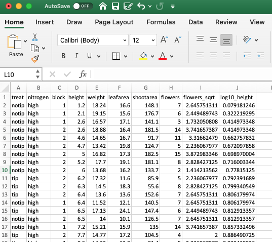
We can of course export our files in a variety of other formats. Another popular option is to export files in csv (comma separated values) format. We can do this using the write.table() function by setting the separator argument to sep = ",".
write.table(flowers_df2, file = 'data/flowers_04_12.csv', col.names = TRUE,
             row.names = FALSE, sep = ",")
Or alternatively by using the convenience function write.csv(). Notice that we don’t need to set the sep = "," or col.names = TRUE arguments as these are the defaults when using the read.csv() function.
write.csv(flowers_df2, file = 'data/flowers_04_12.csv', row.names = FALSE)Other export functions
As with importing data files into R, there are also many alternative functions for exporting data to external files beyond the write.table() function. If you followed the ‘Other import functions’ section of this Chapter you will already have the required packages installed.
The fwrite() function from the data.table package is very efficient at exporting large data objects and is much faster than the write.table() function. It’s also quite simple to use as it has most of the same arguments as write.table(). To export a tab delimited text file we just need to specify the data frame name, the output file name and file path and the separator between columns.
library(data.table)
fwrite(flowers_df2, file = 'data/flowers_04_12.txt', sep = "\t")
To export a csv delimited file it’s even easier as we don’t even need to include the sep = argument.
library(data.table)
fwrite(flowers_df2, file = 'data/flowers_04_12.csv')
The readr package also comes with two useful functions for quickly writing data to external files: the write_tsv() function for writing tab delimited files and the write_csv() function for saving comma separated values (csv) files.
library(readr)
write_tsv(flowers_df2, file = 'data/flowers_04_12.txt')

write_csv(flowers_df2, file = 'data/flowers_04_12.csv')
You can even save data directly to an Excel spreadsheet using the write_excel_csv() function but again we don’t recommend this!