Let’s go through the process of performing logistic regression in R using your provided dataset. I’ll guide you through each step, including data preparation, checking assumptions, model building, and interpretation.
1. Reading the Data
First, load the necessary libraries and read the data from the Excel file.
In this section, we begin by loading the necessary R libraries required for data manipulation, visualization, and model building. The dataset is then imported from an Excel file and briefly examined to understand its structure. The dataset includes variables such as Gender, Hypertension (HT), BMI group, Diabetes Mellitus (DM), and Age group, which will be used to build the logistic regression model.
# Load necessary librarieslibrary(readxl) # For reading Excel fileslibrary(dplyr) # For data manipulation
Attaching package: 'dplyr'
The following objects are masked from 'package:stats':

    filter, lag
The following objects are masked from 'package:base':

    intersect, setdiff, setequal, union
library(tidyr) # For tidy datalibrary(car) # For assumptions testing
Loading required package: carData
Attaching package: 'car'
The following object is masked from 'package:dplyr':

    recode
library(ggplot2) # For data visualizationlibrary(caret) # For model validation
Loading required package: lattice
library(pROC) # For ROC Plots
Type 'citation("pROC")' for a citation.
Attaching package: 'pROC'
The following objects are masked from 'package:stats':

    cov, smooth, var
library(broom) # For tidying up model outputs
Now libraries are loaded. Let’s Read the data.
df <-read_excel("data/LR-Data.xlsx")# View the first few rows of the datahead(df)
The dataset consists of 217 observations and includes categorical variables like Gender and binary variables such as Hypertension and Diabetes Mellitus. Each variable is expected to influence the likelihood of the presence of Diabetes Mellitus, which is our outcome of interest.
Variables Description:
Sl_No: Serial number of the observations.
Gender: Categorical variable indicating the gender of the individual.
1 might represent “Male.”
2 might represent “Female.”
HT: Binary variable indicating the presence of Hypertension (HT).
2.00, 3.00, etc., could represent different BMI groups.
DM: Binary variable indicating the presence of Diabetes Mellitus (DM).
0 indicates “No.”
1 indicates “Yes.”
Agegroup1: Categorical variable representing different age groups.
1.00, 2.00, 3.00, etc., might represent different age ranges.
2. Descriptive Statistics
Next, you want to explore the dataset to understand its basic features. Summary statistics of the dataset are provided to give an overview of the distribution of each variable. This includes the minimum, maximum, mean, and quartiles for continuous and categorical variables.
# Summary statistics of the datasetsummary(df)
     Sl_No           Gender            HT           BMIgroup1
 Min.   :  1.0   Min.   :1.000   Min.   :0.0000   Min.   :1.000
 1st Qu.: 55.0   1st Qu.:1.000   1st Qu.:0.0000   1st Qu.:2.000
 Median :110.0   Median :2.000   Median :1.0000   Median :3.000
 Mean   :109.7   Mean   :1.576   Mean   :0.5438   Mean   :2.433
 3rd Qu.:164.0   3rd Qu.:2.000   3rd Qu.:1.0000   3rd Qu.:3.000
 Max.   :219.0   Max.   :2.000   Max.   :1.0000   Max.   :3.000
       DM          Agegroup1
 Min.   :0.000   Min.   :1.000
 1st Qu.:0.000   1st Qu.:2.000
 Median :1.000   Median :2.000
 Mean   :0.682   Mean   :2.184
 3rd Qu.:1.000   3rd Qu.:3.000
 Max.   :1.000   Max.   :3.000
# Proportion of the outcome variable (DM)print('Proportion of the outcome variable (DM)')
[1] "Proportion of the outcome variable (DM)"
table(df$DM) /nrow(df)
        0         1
0.3179724 0.6820276
The descriptive statistics offer insights into the central tendency and spread of the data. For instance, the average age group is around 2.18, and approximately 68% of the participants have Diabetes Mellitus. Understanding these distributions helps in assessing the model’s inputs and potential impacts.
3. Visualizing the Data
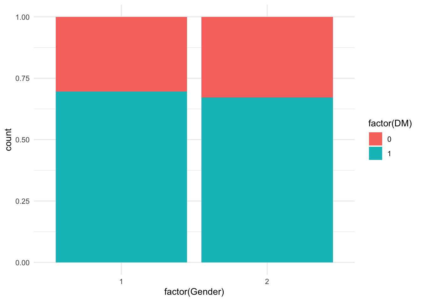
Visualizing the relationships between the predictor variables and the outcome variable is important. Various plots, including histograms and boxplots, are used to visualize the distribution of numeric predictors and their relationship with the outcome variable, Diabetes Mellitus (DM). Bar plots are used for categorical predictors like Gender.
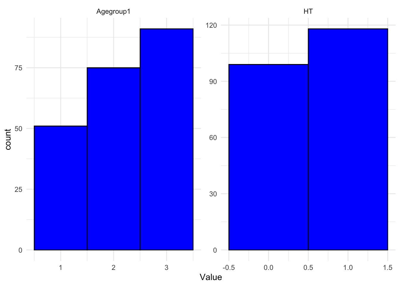
# Plotting histograms for numeric predictors (in this case, HT and Agegroup1)df %>%select(HT, Agegroup1) %>%gather(key ="Variable", value ="Value") %>%ggplot(aes(x = Value)) +facet_wrap(~Variable, scales ="free") +geom_histogram(binwidth =1, fill ="blue", color ="black") +theme_minimal()
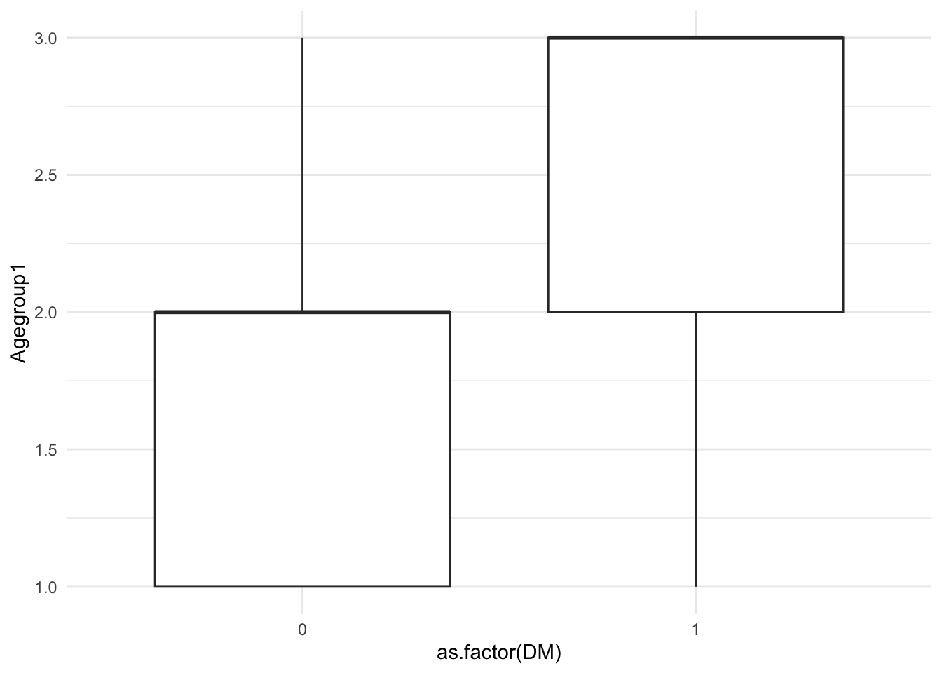
# Boxplot of 'Agegroup1' against 'DM'ggplot(df, aes(x =as.factor(DM), y = Agegroup1)) +geom_boxplot() +theme_minimal()
# Bar plot for categorical predictors (Gender)ggplot(df, aes(x =factor(Gender), fill =factor(DM))) +geom_bar(position ="fill") +theme_minimal()
The visualizations reveal the distribution and potential relationships between predictors and the outcome. For example, histograms show the spread of age groups, while boxplots might indicate a higher age group among those with Diabetes Mellitus. Such insights are crucial for deciding which variables to include in the model.
4. Checking Assumptions
a. Linearity of Logits
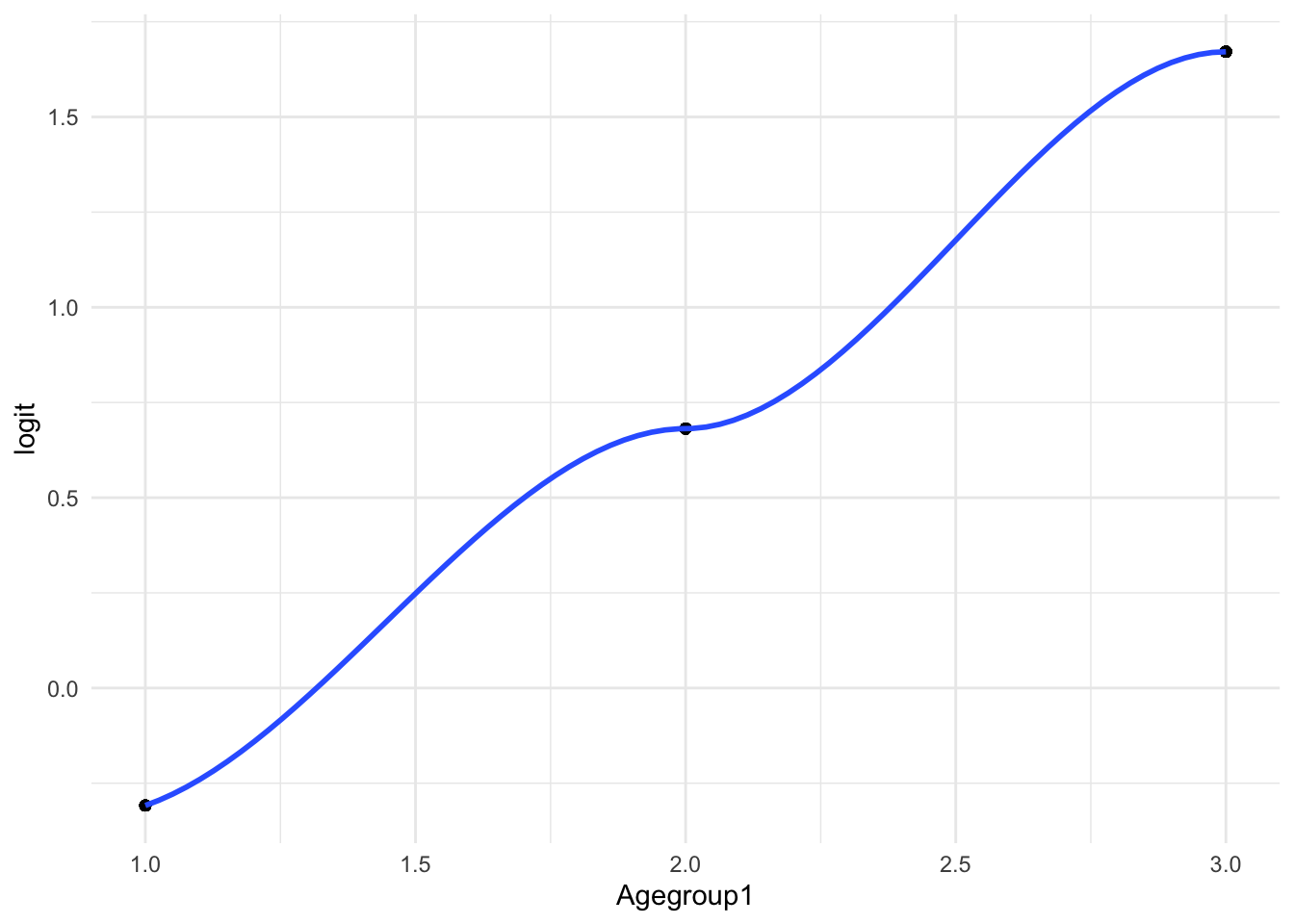
The linearity assumption is checked by plotting the logit of the probability of the outcome against a continuous predictor (Age group). The logit transformation helps in assessing whether the relationship between the predictor and the log odds of the outcome is linear.
# Check linearity for 'Agegroup1' with respect to 'DM'model <-glm(DM ~ Agegroup1, data = df, family = binomial)# Create the logit variabledf <- df %>%mutate(logit =log(predict(model, type ="response") / (1-predict(model, type ="response"))))# Plot the logit against 'Agegroup1'ggplot(df, aes(x = Agegroup1, y = logit)) +geom_point() +geom_smooth(method ="loess") +theme_minimal()
`geom_smooth()` using formula = 'y ~ x'
Warning in simpleLoess(y, x, w, span, degree = degree, parametric = parametric,
: pseudoinverse used at 0.99
Warning in simpleLoess(y, x, w, span, degree = degree, parametric = parametric,
: reciprocal condition number 1.0755e-15
Warning in simpleLoess(y, x, w, span, degree = degree, parametric = parametric,
: There are other near singularities as well. 1.0201
Warning in predLoess(object$y, object$x, newx = if (is.null(newdata)) object$x
else if (is.data.frame(newdata))
as.matrix(model.frame(delete.response(terms(object)), : pseudoinverse used at
0.99
Warning in predLoess(object$y, object$x, newx = if (is.null(newdata)) object$x
else if (is.data.frame(newdata))
as.matrix(model.frame(delete.response(terms(object)), : neighborhood radius
2.01
Warning in predLoess(object$y, object$x, newx = if (is.null(newdata)) object$x
else if (is.data.frame(newdata))
as.matrix(model.frame(delete.response(terms(object)), : reciprocal condition
number 1.0755e-15
Warning in predLoess(object$y, object$x, newx = if (is.null(newdata)) object$x
else if (is.data.frame(newdata))
as.matrix(model.frame(delete.response(terms(object)), : There are other near
singularities as well. 1.0201
If the logit plot reveals a linear trend, it supports the assumption of linearity, making the logistic regression model more reliable. Deviations from linearity might suggest the need for variable transformation or different modeling approaches.
b. Multicollinearity
Multicollinearity among predictors is assessed using the Variance Inflation Factor (VIF). High VIF values indicate multicollinearity, which can affect the model’s estimates.
# Check for multicollinearity using VIFmodel <-glm(DM ~ HT + BMIgroup1 + Agegroup1 + Gender, data = df, family = binomial)vif(model)
The VIF values for all predictors are below the commonly accepted threshold (usually 5 or 10), indicating that multicollinearity is not a concern in this model. This suggests that the estimates for the predictors should be stable and reliable.
5. Model Building
A logistic regression model is built using predictors like Hypertension, BMI group, Age group, and Gender to predict the presence of Diabetes Mellitus. The model’s coefficients are estimated using the maximum likelihood estimation.
# Build the logistic regression modelmodel <-glm(DM ~ HT + BMIgroup1 + Agegroup1 + Gender, data = df, family = binomial)# Summary of the modelsummary(model)
Call:
glm(formula = DM ~ HT + BMIgroup1 + Agegroup1 + Gender, family = binomial,
    data = df)

Coefficients:
            Estimate Std. Error z value Pr(>|z|)
(Intercept)  -3.7897     0.9904  -3.826 0.000130 ***
HT            1.0947     0.3588   3.051 0.002278 **
BMIgroup1     1.0408     0.2775   3.750 0.000177 ***
Agegroup1     0.8544     0.2322   3.680 0.000233 ***
Gender       -0.1412     0.3435  -0.411 0.681049
---
Signif. codes:  0 '***' 0.001 '**' 0.01 '*' 0.05 '.' 0.1 ' ' 1

(Dispersion parameter for binomial family taken to be 1)

    Null deviance: 271.39  on 216  degrees of freedom
Residual deviance: 217.49  on 212  degrees of freedom
AIC: 227.49

Number of Fisher Scoring iterations: 4
The model shows that Hypertension, BMI group, and Age group are significant predictors of Diabetes Mellitus, as indicated by their p-values. Gender does not appear to be a significant predictor in this model. The coefficients represent the log odds of having Diabetes Mellitus for a one-unit increase in each predictor, holding other variables constant.
6. Model Validation
Cross-validation is employed to assess the stability and generalizability of the model. The model’s performance is evaluated across multiple folds of the data to avoid overfitting.
# Set up cross-validationtrain_control <-trainControl(method ="cv", number =10)# Train the model with cross-validationmodel_cv <-train(DM ~ HT + BMIgroup1 + Agegroup1 + Gender, data = df, method ="glm", family ="binomial", trControl = train_control)
Warning in train.default(x, y, weights = w, ...): You are trying to do
regression and your outcome only has two possible values Are you trying to do
classification? If so, use a 2 level factor as your outcome column.
# Summary of cross-validated modelsummary(model_cv)
Call:
NULL

Coefficients:
            Estimate Std. Error z value Pr(>|z|)
(Intercept)  -3.7897     0.9904  -3.826 0.000130 ***
HT            1.0947     0.3588   3.051 0.002278 **
BMIgroup1     1.0408     0.2775   3.750 0.000177 ***
Agegroup1     0.8544     0.2322   3.680 0.000233 ***
Gender       -0.1412     0.3435  -0.411 0.681049
---
Signif. codes:  0 '***' 0.001 '**' 0.01 '*' 0.05 '.' 0.1 ' ' 1

(Dispersion parameter for binomial family taken to be 1)

    Null deviance: 271.39  on 216  degrees of freedom
Residual deviance: 217.49  on 212  degrees of freedom
AIC: 227.49

Number of Fisher Scoring iterations: 4
The cross-validated model shows an accuracy of approximately 75.6%, with a balanced accuracy of 70.1%. These metrics suggest that the model performs reasonably well in predicting Diabetes Mellitus, but there may still be room for improvement.
7. Odds Ratios
Odds ratios and their confidence intervals are calculated to interpret the effect size of each predictor in the logistic regression model.
# Calculate odds ratios and confidence intervalsexp(cbind(OR =coef(model), confint(model)))
The odds ratios indicate that individuals with Hypertension have approximately 3 times higher odds of having Diabetes Mellitus. Similarly, higher BMI groups and older age groups are associated with increased odds of Diabetes Mellitus, highlighting these as important risk factors.
8. Model Prediction
Predicted probabilities and outcomes are generated based on the logistic regression model. A confusion matrix is used to evaluate the model’s classification performance.
Confusion Matrix and Statistics

          Reference
Prediction   0   1
         0  38  22
         1  31 126

               Accuracy : 0.7558
                 95% CI : (0.693, 0.8114)
    No Information Rate : 0.682
    P-Value [Acc > NIR] : 0.01066

                  Kappa : 0.4166

 Mcnemar's Test P-Value : 0.27182

            Sensitivity : 0.5507
            Specificity : 0.8514
         Pos Pred Value : 0.6333
         Neg Pred Value : 0.8025
             Prevalence : 0.3180
         Detection Rate : 0.1751
   Detection Prevalence : 0.2765
      Balanced Accuracy : 0.7010

       'Positive' Class : 0
The model correctly classifies about 75.6% of the cases, with higher specificity (85.1%) than sensitivity (55.1%). This suggests the model is better at identifying those without Diabetes Mellitus but less accurate at identifying those with the condition.
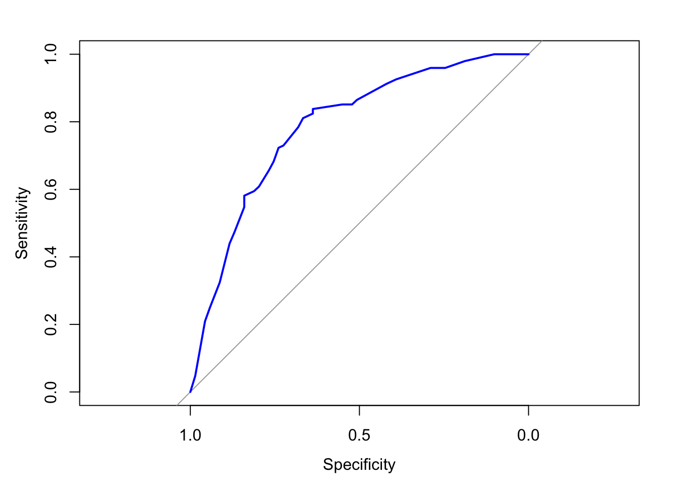
9. ROC Curve
The ROC curve is plotted to evaluate the model’s ability to discriminate between those with and without Diabetes Mellitus. The Area Under the Curve (AUC) is also calculated.
The AUC of 0.7863 indicates that the model has a good ability to distinguish between individuals with and without Diabetes Mellitus. AUC values closer to 1.0 indicate better discrimination.
10. Model Interpretation
This section synthesizes the results of the logistic regression analysis, discussing the implications of the significant predictors and the overall model performance.
The model identifies key risk factors for Diabetes Mellitus, such as Hypertension, BMI, and Age group, which can be useful for targeted interventions. However, the model’s moderate accuracy and sensitivity suggest that additional predictors or alternative modeling approaches may be needed to improve performance.